梯度下降（Gradient Descent）是深度学习中最核心的优化算法之一。大模型（如GPT、BERT）在训练时需要优化数十亿甚至上千亿的参数，而梯度下降及其变体（如SGD、Adam）正是实现这一优化的关键工具。它通过计算损失函数相对于参数的梯度，并沿梯度负方向迭代更新参数，从而最小化损失。

梯度下降解决的问题

在大模型训练中，我们需要最小化一个高维、非凸的损失函数。梯度下降的目标就是找到损失函数的局部甚至全局最优点，以使模型在训练数据和测试数据上表现良好。

主要解决的问题包括：

损失最小化：通过迭代不断减少模型预测与真实值之间的误差。

收敛效率：改进的优化算法（如Adam）可以加速收敛。

避免困在鞍点：高维空间中鞍点比局部极小值更常见，因此优化器需具备跳出鞍点的能力。

2. 原理与数学推导

2.1 基本公式

梯度下降的更新规则为：

公式如下：

$${\theta }_{t+1}={\theta }_t-\eta \cdot {\nabla }_{\theta }L({\theta }_t)$$

其中：

• $\theta$ 是模型参数；
• $L(\theta )$ 是损失函数；
• $\eta$ 是学习率（Learning Rate）；
• ${\nabla }_{\theta }L$ 是损失函数对参数的梯度。

---

2.2 损失函数的几何意义

损失函数可以看作一个“地形”，梯度下降就是沿着最陡峭的下坡路一步步走到山谷底部（全局或局部最小值）。

---

3. 梯度下降的种类与应用

算法	特点	适用场景
Batch GD	使用全量数据，稳定但计算量大	小数据集
SGD	每次用一个样本，更新快但噪声大	深度学习初期
Mini-Batch GD	折中方案，批量样本	大模型训练首选

---

4. 在大模型训练中的实践

• 优化器：Adam / AdamW 广泛用于 LLM 训练；
• Loss：交叉熵（Cross Entropy）是语言建模的常见选择；
• 技巧：学习率调度（Warm-up）、梯度裁剪（Gradient Clipping）、正则化（Weight Decay）。

---

5. 可视化示例：梯度下降过程

以下示例演示了如何用 Python + Matplotlib 画出梯度下降在二维损失曲面上的收敛轨迹。

import numpy as np
import matplotlib.pyplot as plt# 损失函数: f(x) = x^2 + 2x + 1
def loss(x):return x**2 + 2*x + 1# 梯度: f'(x) = 2x + 2
def grad(x):return 2*x + 2# 参数初始化
x = 5.0
eta = 0.2  # 学习率
history = [x]# 迭代梯度下降
for _ in range(15):x -= eta * grad(x)history.append(x)# 绘图
xs = np.linspace(-4, 6, 100)
ys = loss(xs)plt.figure(figsize=(8,4))
plt.plot(xs, ys, label="Loss Curve")
plt.scatter(history, [loss(h) for h in history], c="red", label="Steps", zorder=5)
plt.title("Gradient Descent Optimization Path")
plt.xlabel("Parameter x")
plt.ylabel("Loss")
plt.legend()
plt.grid(True)
plt.show()

运行后会显示：

• 蓝色曲线：损失函数 $L(x)=x^2+2x+1$
• 红点：梯度下降的更新轨迹，逐步逼近最小值。

---

6. 图示（直观理解）

损失 L(θ)
│       •            ← 初始参数 θ0
│     •
│   •
│ •
└──────────────────────────→ 参数 θ

---

7. 示例：PyTorch 训练循环（简化版）

import torch
import torch.nn as nn
import torch.optim as optim# 简单线性模型 y = wx + b
model = nn.Linear(1, 1)
criterion = nn.MSELoss()
optimizer = optim.AdamW(model.parameters(), lr=0.01)x = torch.randn(100, 1)
y = 3 * x + 1 + 0.1 * torch.randn(100, 1)for epoch in range(100):optimizer.zero_grad()y_pred = model(x)loss = criterion(y_pred, y)loss.backward()optimizer.step()if epoch % 10 == 0:print(f"Epoch {epoch}: Loss = {loss.item():.4f}")

这段代码模拟了一个使用 AdamW + MSE Loss 的小型训练过程。

7. Jupyter Notebook详细版本

可视化与轨迹演示的demo示意

pip install numpy matplotlib torch pillow

import matplotlib
matplotlib.rcParams['font.sans-serif'] = ['Arial Unicode MS', 'SimHei']  # Mac/Windows 中文字体
matplotlib.rcParams['axes.unicode_minus'] = Falseimport numpy as np
import matplotlib.pyplot as plt
import matplotlib.animation as animation
import torch
import torch.nn as nn
import torch.optim as optim#############################
# 1. 一维梯度下降动画
#############################def loss_1d(x):return x**2 + 2*x + 1def grad_1d(x):return 2*x + 2x_init = 5.0
eta = 0.2
steps = [x_init]
x = x_init
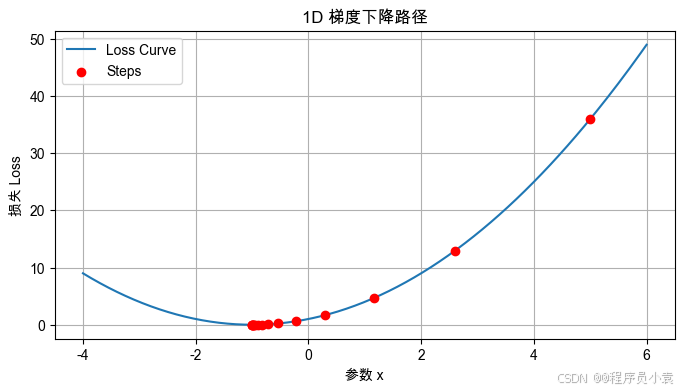
for _ in range(15):x -= eta * grad_1d(x)steps.append(x)xs = np.linspace(-4, 6, 200)
ys = loss_1d(xs)
plt.figure(figsize=(8,4))
plt.plot(xs, ys, label="Loss Curve")
plt.scatter(steps, [loss_1d(s) for s in steps], c="red", label="Steps", zorder=5)
plt.title("1D 梯度下降路径")
plt.xlabel("参数 x")
plt.ylabel("损失 Loss")
plt.legend()
plt.grid(True)
plt.show()fig, ax = plt.subplots()
ax.plot(xs, ys, label="Loss Curve")
point, = ax.plot([], [], 'ro')
ax.legend()
ax.set_title("1D 梯度下降动画")
ax.set_xlabel("参数 x")
ax.set_ylabel("损失 Loss")def init():point.set_data([], [])return point,def update(frame):x_val = steps[frame]y_val = loss_1d(x_val)point.set_data([x_val], [y_val])return point,ani = animation.FuncAnimation(fig, update, frames=len(steps), init_func=init, blit=True)
plt.close(fig)
ani.save("gradient_descent_1d.gif", writer="pillow", fps=2)#############################
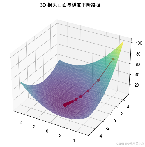
# 2. 三维损失曲面 + 路径
#############################def loss_2d(w):x, y = wreturn x**2 + y**2 + x*y + 2*x + 3*y + 5def grad_2d(w):x, y = wreturn np.array([2*x + y + 2, 2*y + x + 3])eta = 0.1
w = np.array([4.0, 4.0])
path = [w.copy()]
for _ in range(30):w -= eta * grad_2d(w)path.append(w.copy())X = np.linspace(-5, 5, 50)
Y = np.linspace(-5, 5, 50)
X, Y = np.meshgrid(X, Y)
Z = loss_2d([X, Y])fig = plt.figure(figsize=(8,6))
ax = fig.add_subplot(111, projection='3d')
ax.plot_surface(X, Y, Z, cmap='viridis', alpha=0.7)
path = np.array(path)
ax.plot(path[:,0], path[:,1], [loss_2d(p) for p in path], 'r-o')
ax.set_title("3D 损失曲面与梯度下降路径")
plt.show()#############################
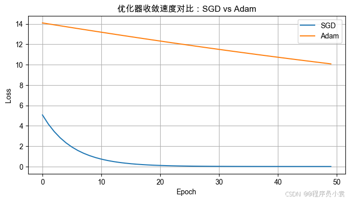
# 3. 优化器对比：SGD vs Adam
#############################torch.manual_seed(0)
X = torch.randn(200,1)
y = 3*X + 1 + 0.1*torch.randn(200,1)def build_model():return nn.Linear(1,1)def train(optimizer_type, lr=0.01):model = build_model()criterion = nn.MSELoss()optimizer = optimizer_type(model.parameters(), lr=lr)losses = []for epoch in range(50):optimizer.zero_grad()y_pred = model(X)loss = criterion(y_pred, y)loss.backward()optimizer.step()losses.append(loss.item())return lossesloss_sgd = train(optim.SGD, lr=0.05)
loss_adam = train(optim.Adam, lr=0.01)plt.figure(figsize=(8,4))
plt.plot(loss_sgd, label="SGD")
plt.plot(loss_adam, label="Adam")
plt.xlabel("Epoch")
plt.ylabel("Loss")
plt.title("优化器收敛速度对比：SGD vs Adam")
plt.legend()
plt.grid(True)
plt.show()