前言：前文分享了注意力机制，今天开始分享案例：seqtoseq英译法。

一、案例概述

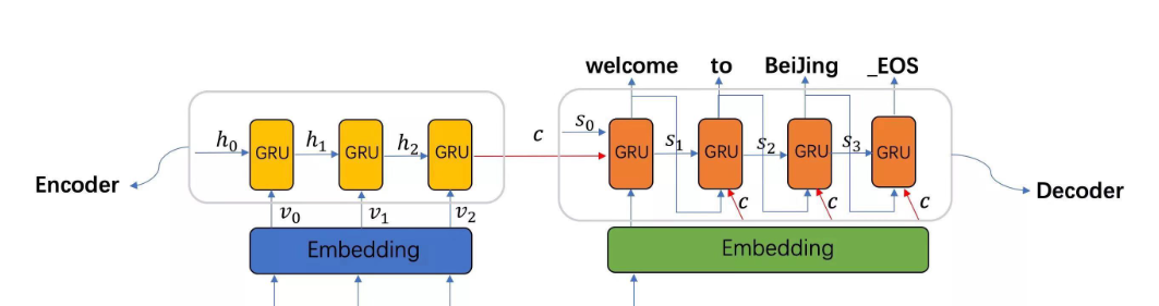
任务：将英文短句翻译成法文（例如：“I am happy.” → “Je suis heureux.”）

模型架构：Seq2Seq 带注意力机制（Attention）

二、数据集

i am from brazil .  je viens du bresil .
i am from france .  je viens de france .
i am from russia .  je viens de russie .
i am frying fish .  je fais frire du poisson .
i am not kidding .  je ne blague pas .
i am on duty now .  maintenant je suis en service .
i am on duty now .  je suis actuellement en service .
i am only joking .  je ne fais que blaguer .
i am out of time .  je suis a court de temps .
i am out of work .  je suis au chomage .
i am out of work .  je suis sans travail .
i am paid weekly .  je suis payee a la semaine .
i am pretty sure .  je suis relativement sur .
i am truly sorry .  je suis vraiment desole .
i am truly sorry .  je suis vraiment desolee .

三、案例步骤

基于GRU的seq2seq模型架构实现翻译的过程:

第一步: 导入工具包和工具函数；
第二步: 对持久化文件中数据进行处理, 以满足模型训练要求；
第三步: 构建基于GRU的编码器和解码器；
第四步: 构建模型训练函数, 并进行训练；
第五步: 构建模型评估函数, 并进行测试以及Attention效果分析。

（一）导入工具包和工具函数

# 用于正则表达式
import re
# 用于构建网络结构和函数的torch工具包
import torch
import torch.nn as nn
import torch.nn.functional as F
from torch.utils.data import Dataset, DataLoader
# torch中预定义的优化方法工具包
import torch.optim as optim
import time
# 用于随机生成数据
import random
import matplotlib.pyplot as plt# 设备选择, 我们可以选择在cuda或者cpu上运行你的代码
device = torch.device("cuda" if torch.cuda.is_available() else "cpu")
# 起始标志
SOS_token = 0
# 结束标志
EOS_token = 1
# 最大句子长度不能超过10个 (包含标点)
MAX_LENGTH = 10
# 数据文件路径
data_path = './data/eng-fra-v2.txt'# 文本清洗工具函数
def normalizeString(s):"""字符串规范化函数, 参数s代表传入的字符串"""s = s.lower().strip()# 在.!?前加一个空格  这里的\1表示第一个分组   正则中的\nums = re.sub(r"([.!?])", r" \1", s)# s = re.sub(r"([.!?])", r" ", s)# 使用正则表达式将字符串中 不是 大小写字母和正常标点的都替换成空格s = re.sub(r"[^a-zA-Z.!?]+", r" ", s)return s

（二）数据预处理

def my_getdata():# 1 按行读文件 open().read().strip().split(\n)my_lines = open(data_path, encoding='utf-8').read().strip().split('\n')print('my_lines--->', len(my_lines))# 2 按行清洗文本 构建语言对 my_pairs# 格式 [['英文句子', '法文句子'], ['英文句子', '法文句子'], ['英文句子', '法文句子'], ... ]# tmp_pair, my_pairs = [], []# for l in my_lines:#     for s in l.split('\t'):#         tmp_pair.append(normalizeString(s))#     my_pairs.append(tmp_pair)#     tmp_pair = []my_pairs = [[normalizeString(s) for s in l.split('\t')] for l in my_lines]print('len(pairs)--->', len(my_pairs))# 打印前4条数据print(my_pairs[:4])# 打印第8000条的英文 法文数据print('my_pairs[8000][0]--->', my_pairs[8000][0])print('my_pairs[8000][1]--->', my_pairs[8000][1])# 3 遍历语言对 构建英语单词字典 法语单词字典# 3-1 english_word2index english_word_n french_word2index french_word_nenglish_word2index = {"SOS": 0, "EOS": 1}english_word_n = 2french_word2index = {"SOS": 0, "EOS": 1}french_word_n = 2# 遍历语言对 获取英语单词字典 法语单词字典for pair in my_pairs:for word in pair[0].split(' '):if word not in english_word2index:english_word2index[word] = english_word_nenglish_word_n += 1for word in pair[1].split(' '):if word not in french_word2index:french_word2index[word] = french_word_nfrench_word_n += 1# 3-2 english_index2word french_index2wordenglish_index2word = {v:k for k, v in english_word2index.items()}french_index2word = {v:k for k, v in french_word2index.items()}print('len(english_word2index)-->', len(english_word2index))print('len(french_word2index)-->', len(french_word2index))print('english_word_n--->', english_word_n, 'french_word_n-->', french_word_n)return english_word2index, english_index2word, english_word_n, french_word2index, french_index2word, french_word_n, my_pairs

运行结果：

my_lines---> 10599
len(pairs)---> 10599
[['i m .', 'j ai ans .'], ['i m ok .', 'je vais bien .'], ['i m ok .', 'ca va .'], ['i m fat .', 'je suis gras .']]
my_pairs[8000][0]---> they re in the science lab .
my_pairs[8000][1]---> elles sont dans le laboratoire de sciences .
len(english_word2index)--> 2803
len(french_word2index)--> 4345
english_word_n---> 2803 french_word_n--> 4345
x.shape torch.Size([1, 9]) tensor([[ 75,  40, 102, 103, 677,  42,  21,   4,   1]])
y.shape torch.Size([1, 7]) tensor([[ 119,   25,  164,  165, 3222,    5,    1]])
x.shape torch.Size([1, 5]) tensor([[14, 15, 44,  4,  1]])
y.shape torch.Size([1, 5]) tensor([[24, 25, 62,  5,  1]])
x.shape torch.Size([1, 8]) tensor([[   2,    3,  147,   61,  532, 1143,    4,    1]])
y.shape torch.Size([1, 7]) tensor([[  6, 297,   7, 246, 102,   5,   1]])

（三）构建数据源对象

# 原始数据 -> 数据源MyPairsDataset --> 数据迭代器DataLoader
# 构造数据源 MyPairsDataset，把语料xy 文本数值化 再转成tensor_x tensor_y
# 1 __init__(self, my_pairs)函数 设置self.my_pairs 条目数self.sample_len
# 2 __len__(self)函数  获取样本条数
# 3 __getitem__(self, index)函数 获取第几条样本数据
#       按索引 获取数据样本 x y
#       样本x 文本数值化   word2id  x.append(EOS_token)
#       样本y 文本数值化   word2id  y.append(EOS_token)
#       返回tensor_x, tensor_yclass MyPairsDataset(Dataset):def __init__(self, my_pairs):# 样本xself.my_pairs = my_pairs# 样本条目数self.sample_len = len(my_pairs)# 获取样本条数def __len__(self):return self.sample_len# 获取第几条 样本数据def __getitem__(self, index):# 对index异常值进行修正 [0, self.sample_len-1]index = min(max(index, 0), self.sample_len-1)# 按索引获取 数据样本 x yx = self.my_pairs[index][0]y = self.my_pairs[index][1]# 样本x 文本数值化x = [english_word2index[word] for word in x.split(' ')]x.append(EOS_token)tensor_x = torch.tensor(x, dtype=torch.long, device=device)# 样本y 文本数值化y = [french_word2index[word] for word in y.split(' ')]y.append(EOS_token)tensor_y = torch.tensor(y, dtype=torch.long, device=device)# 注意 tensor_x tensor_y都是一维数组，通过DataLoader拿出数据是二维数据# print('tensor_y.shape===>', tensor_y.shape, tensor_y)# 返回结果return tensor_x, tensor_y

（四）构建数据迭代器

def dm_test_MyPairsDataset():# 1 实例化dataset对象mypairsdataset = MyPairsDataset(my_pairs)# 2 实例化dataloadermydataloader = DataLoader(dataset=mypairsdataset, batch_size=1, shuffle=True)for  i, (x, y) in enumerate (mydataloader):print('x.shape', x.shape, x)print('y.shape', y.shape, y)if i == 1:break

运行结果：

x.shape torch.Size([1, 8]) tensor([[   2,   16,   33,  518,  589, 1460,    4,    1]])
y.shape torch.Size([1, 8]) tensor([[   6,   11,   52,  101, 1358,  964,    5,    1]])
x.shape torch.Size([1, 6]) tensor([[129,  78, 677, 429,   4,   1]])
y.shape torch.Size([1, 7]) tensor([[ 118,  214, 1073,  194,  778,    5,    1]])

（五）构建基于GRU的编码器和解码器

1.构建基于GRU的编码器

编码器结构图:

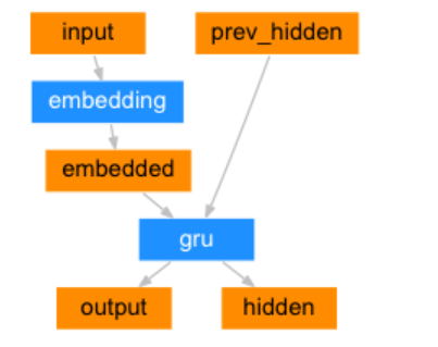
class EncoderRNN(nn.Module):def __init__(self, input_size, hidden_size):# input_size 编码器 词嵌入层单词数 eg：2803# hidden_size 编码器 词嵌入层每个单词的特征数 eg 256super(EncoderRNN, self).__init__()self.input_size = input_sizeself.hidden_size = hidden_size# 实例化nn.Embedding层self.embedding = nn.Embedding(input_size, hidden_size)# 实例化nn.GRU层 注意参数batch_first=Trueself.gru = nn.GRU(hidden_size, hidden_size, batch_first=True)def forward(self, input, hidden):# 数据经过词嵌入层 数据形状 [1,6] --> [1,6,256]output = self.embedding(input)# 数据经过gru层 数据形状 gru([1,6,256],[1,1,256]) --> [1,6,256] [1,1,256]output, hidden = self.gru(output, hidden)return output, hiddendef inithidden(self):# 将隐层张量初始化成为1x1xself.hidden_size大小的张量return torch.zeros(1, 1, self.hidden_size, device=device)

调用：

def dm_test_EncoderRNN():# 实例化dataset对象mypairsdataset = MyPairsDataset(my_pairs)# 实例化dataloadermydataloader = DataLoader(dataset=mypairsdataset, batch_size=1, shuffle=True)# 实例化模型input_size = english_word_nhidden_size = 256 #my_encoderrnn = EncoderRNN(input_size, hidden_size)print('my_encoderrnn模型结构--->', my_encoderrnn)# 给encode模型喂数据for  i, (x, y) in enumerate (mydataloader):print('x.shape', x.shape, x)print('y.shape', y.shape, y)# 一次性的送数据hidden = my_encoderrnn.inithidden()encode_output_c, hidden = my_encoderrnn(x, hidden)print('encode_output_c.shape--->', encode_output_c.shape, encode_output_c)# 一个字符一个字符给为模型喂数据hidden = my_encoderrnn.inithidden()for i in range(x.shape[1]):tmp = x[0][i].view(1,-1)output, hidden = my_encoderrnn(tmp, hidden)print('观察：最后一个时间步output输出是否相等') # hidden_size = 8 效果比较好print('encode_output_c[0][-1]===>', encode_output_c[0][-1])print('output===>', output)break

输出效果:

# 本输出效果为hidden_size = 8
x.shape torch.Size([1, 6]) tensor([[129, 124, 270, 558,   4,   1]])
y.shape torch.Size([1, 7]) tensor([[ 118,  214,  101, 1253, 1028,    5,    1]])
encode_output_c.shape---> torch.Size([1, 6, 8]) 
tensor([[[-0.0984,  0.4267, -0.2120,  0.0923,  0.1525, -0.0378,  0.2493,-0.2665],[-0.1388,  0.5363, -0.4522, -0.2819, -0.2070,  0.0795,  0.6262, -0.2359],[-0.4593,  0.2499,  0.1159,  0.3519, -0.0852, -0.3621,  0.1980, -0.1853],[-0.4407,  0.1974,  0.6873, -0.0483, -0.2730, -0.2190,  0.0587, 0.2320],[-0.6544,  0.1990,  0.7534, -0.2347, -0.0686, -0.5532,  0.0624, 0.4083],[-0.2941, -0.0427,  0.1017, -0.1057,  0.1983, -0.1066,  0.0881, -0.3936]]], grad_fn=<TransposeBackward1>)
观察：最后一个时间步output输出是否相等
encode_output_c[0][-1]===> tensor([-0.2941, -0.0427,  0.1017, -0.1057,  0.1983, -0.1066,  0.0881, -0.3936],grad_fn=<SelectBackward0>)
output===> tensor([[[-0.2941, -0.0427,  0.1017, -0.1057,  0.1983, -0.1066,  0.0881,-0.3936]]], grad_fn=<TransposeBackward1>)

2. 构建基于GRU的解码器

解码器结构图:

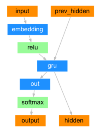
class DecoderRNN(nn.Module):def __init__(self, output_size, hidden_size):# output_size 编码器 词嵌入层单词数 eg：4345# hidden_size 编码器 词嵌入层每个单词的特征数 eg 256super(DecoderRNN, self).__init__()self.output_size = output_sizeself.hidden_size = hidden_size# 实例化词嵌入层self.embedding = nn.Embedding(output_size, hidden_size)# 实例化gru层，输入尺寸256 输出尺寸256# 因解码器一个字符一个字符的解码 batch_first=True 意义不大self.gru = nn.GRU(hidden_size, hidden_size, batch_first=True)# 实例化线性输出层out 输入尺寸256 输出尺寸4345self.out = nn.Linear(hidden_size, output_size)# 实例化softomax层 数值归一化 以便分类self.softmax = nn.LogSoftmax(dim=-1)def forward(self, input, hidden):# 数据经过词嵌入层# 数据形状 [1,1] --> [1,1,256] or [1,6]--->[1,6,256]output = self.embedding(input)# 数据结果relu层使Embedding矩阵更稀疏，以防止过拟合output = F.relu(output)# 数据经过gru层# 数据形状 gru([1,1,256],[1,1,256]) --> [1,1,256] [1,1,256]output, hidden = self.gru(output, hidden)# 数据经过softmax层 归一化# 数据形状变化 [1,1,256]->[1,256] ---> [1,4345]output = self.softmax(self.out(output[0]))return output, hiddendef inithidden(self):# 将隐层张量初始化成为1x1xself.hidden_size大小的张量return torch.zeros(1, 1, self.hidden_size, device=device)

调用：

def dm03_test_DecoderRNN():# 实例化dataset对象mypairsdataset = MyPairsDataset(my_pairs)# 实例化dataloadermydataloader = DataLoader(dataset=mypairsdataset, batch_size=1, shuffle=True)# 实例化模型input_size = english_word_nhidden_size = 256 # 观察结果数据 可使用8my_encoderrnn = EncoderRNN(input_size, hidden_size)print('my_encoderrnn模型结构--->', my_encoderrnn)# 实例化模型input_size = french_word_nhidden_size = 256  # 观察结果数据 可使用8my_decoderrnn = DecoderRNN(input_size, hidden_size)print('my_decoderrnn模型结构--->', my_decoderrnn)# 给模型喂数据 完整演示编码 解码流程for i, (x, y) in enumerate (mydataloader):print('x.shape', x.shape, x)print('y.shape', y.shape, y)# 1 编码：一次性的送数据hidden = my_encoderrnn.inithidden()encode_output_c, hidden = my_encoderrnn(x, hidden)print('encode_output_c.shape--->', encode_output_c.shape, encode_output_c)print('观察：最后一个时间步output输出') # hidden_size = 8 效果比较好print('encode_output_c[0][-1]===>', encode_output_c[0][-1])# 2 解码: 一个字符一个字符的解码# 最后1个隐藏层的输出 作为 解码器的第1个时间步隐藏层输入for i in range(y.shape[1]):tmp = y[0][i].view(1, -1)output, hidden = my_decoderrnn(tmp, hidden)print('每个时间步解码出来4345种可能 output===>', output.shape)break

输出效果：

my_encoderrnn模型结构---> EncoderRNN((embedding): Embedding(2803, 256)(gru): GRU(256, 256, batch_first=True)
)
my_decoderrnn模型结构---> DecoderRNN((embedding): Embedding(4345, 256)(gru): GRU(256, 256, batch_first=True)(out): Linear(in_features=256, out_features=4345, bias=True)(softmax): LogSoftmax(dim=-1)
)
x.shape torch.Size([1, 8]) tensor([[ 14,  40, 883, 677, 589, 609,   4,   1]])
y.shape torch.Size([1, 6]) tensor([[1358, 1125,  247, 2863,    5,    1]])
每个时间步解码出来4345种可能 output===> torch.Size([1, 4345])
每个时间步解码出来4345种可能 output===> torch.Size([1, 4345])
每个时间步解码出来4345种可能 output===> torch.Size([1, 4345])
每个时间步解码出来4345种可能 output===> torch.Size([1, 4345])
每个时间步解码出来4345种可能 output===> torch.Size([1, 4345])
每个时间步解码出来4345种可能 output===> torch.Size([1, 4345])

3 .构建基于GRU和Attention的解码器

解码器结构图:

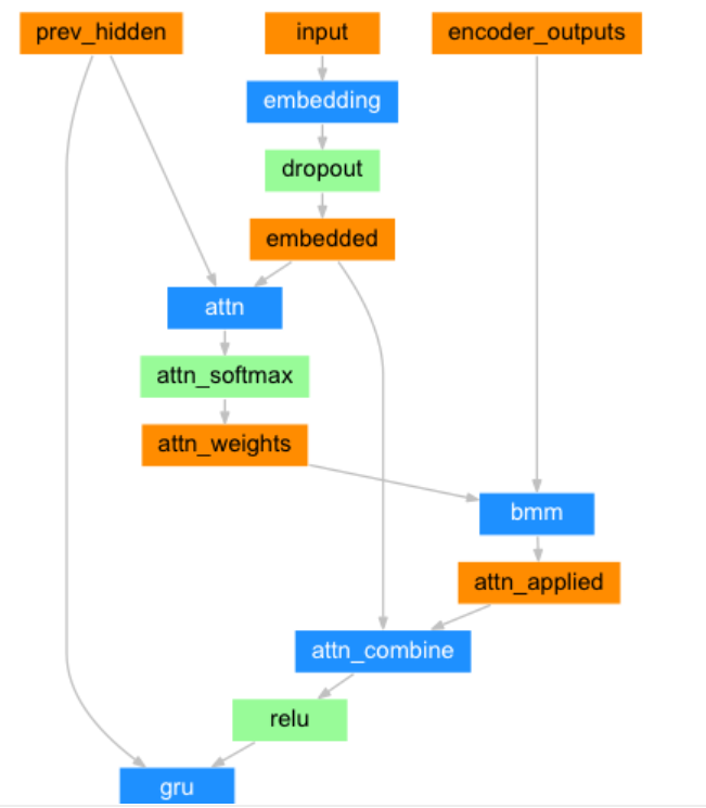
class AttnDecoderRNN(nn.Module):def __init__(self, output_size, hidden_size, dropout_p=0.1, max_length=MAX_LENGTH):# output_size   编码器 词嵌入层单词数 eg：4345# hidden_size   编码器 词嵌入层每个单词的特征数 eg 256# dropout_p     置零比率，默认0.1,# max_length    最大长度10super(AttnDecoderRNN, self).__init__()self.output_size = output_sizeself.hidden_size = hidden_sizeself.dropout_p = dropout_pself.max_length = max_length# 定义nn.Embedding层 nn.Embedding(4345,256)self.embedding = nn.Embedding(self.output_size, self.hidden_size)# 定义线性层1：求q的注意力权重分布self.attn = nn.Linear(self.hidden_size * 2, self.max_length)# 定义线性层2：q+注意力结果表示融合后，在按照指定维度输出self.attn_combine = nn.Linear(self.hidden_size * 2, self.hidden_size)# 定义dropout层self.dropout = nn.Dropout(self.dropout_p)# 定义gru层self.gru = nn.GRU(self.hidden_size, self.hidden_size, batch_first=True)# 定义out层 解码器按照类别进行输出(256,4345)self.out = nn.Linear(self.hidden_size, self.output_size)# 实例化softomax层 数值归一化 以便分类self.softmax = nn.LogSoftmax(dim=-1)def forward(self, input, hidden, encoder_outputs):# input代表q [1,1] 二维数据 hidden代表k [1,1,256] encoder_outputs代表v [10,256]# 数据经过词嵌入层# 数据形状 [1,1] --> [1,1,256]embedded = self.embedding(input)# 使用dropout进行随机丢弃，防止过拟合embedded = self.dropout(embedded)# 1 求查询张量q的注意力权重分布, attn_weights[1,10]attn_weights = F.softmax(self.attn(torch.cat((embedded[0], hidden[0]), 1)), dim=1)# 2 求查询张量q的注意力结果表示 bmm运算, attn_applied[1,1,256]# [1,1,10],[1,10,256] ---> [1,1,256]attn_applied = torch.bmm(attn_weights.unsqueeze(0), encoder_outputs.unsqueeze(0))# 3 q 与 attn_applied 融合，再按照指定维度输出 output[1,1,256]output = torch.cat((embedded[0], attn_applied[0]), 1)output = self.attn_combine(output).unsqueeze(0)# 查询张量q的注意力结果表示 使用relu激活output = F.relu(output)# 查询张量经过gru、softmax进行分类结果输出# 数据形状[1,1,256],[1,1,256] --> [1,1,256], [1,1,256]output, hidden = self.gru(output, hidden)# 数据形状[1,1,256]->[1,256]->[1,4345]output = self.softmax(self.out(output[0]))# 返回解码器分类output[1,4345]，最后隐层张量hidden[1,1,256] 注意力权重张量attn_weights[1,10]return output, hidden, attn_weightsdef inithidden(self):# 将隐层张量初始化成为1x1xself.hidden_size大小的张量return torch.zeros(1, 1, self.hidden_size, device=device)

调用：

def dm_test_AttnDecoderRNN():# 1 实例化 数据集对象mypairsdataset = MyPairsDataset(my_pairs)# 2 实例化 数据加载器对象mydataloader = DataLoader(dataset=mypairsdataset, batch_size=1, shuffle=True)#  实例化 编码器my_encoderrnnmy_encoderrnn = EncoderRNN(english_word_n, 256)# 实例化 解码器DecoderRNNmy_attndecoderrnn = AttnDecoderRNN(french_word_n, 256)# 3 遍历数据迭代器for i, (x, y) in enumerate(mydataloader):# 编码-方法1 一次性给模型送数据hidden = my_encoderrnn.inithidden()print('x--->', x.shape, x)print('y--->', y.shape, y)# [1, 6, 256], [1, 1, 256]) --> [1, 6, 256][1, 1, 256]output, hidden = my_encoderrnn(x, hidden)# print('output-->', output.shape, output)# print('最后一个时间步取出output[0,-1]-->', output[0, -1].shape, output[0, -1])# 中间语义张量Cencode_output_c = torch.zeros(MAX_LENGTH, my_encoderrnn.hidden_size,device=device)for idx in range(output.shape[1]):encode_output_c[idx] = output[0, idx]# # 编码-方法2 一个字符一个字符给模型送数据# hidden = my_encoderrnn.inithidden()# for i in range(x.shape[1]):#     tmp = x[0][i].view(1, -1)#     # [1, 1, 256], [1, 1, 256]) --> [1, 1, 256][1, 1, 256]#     output, hidden = my_encoderrnn(tmp, hidden)# print('一个字符一个字符output', output.shape, output)# 解码-必须一个字符一个字符的解码 for i in range(y.shape[1]):tmp = y[0][i].view(1, -1)output, hidden, attn_weights = my_attndecoderrnn(tmp, hidden, encode_output_c)print('解码output.shape', output.shape )print('解码hidden.shape', hidden.shape)print('解码attn_weights.shape', attn_weights.shape)break

输出效果:

x---> torch.Size([1, 7]) tensor([[ 129,   78, 1873,  294, 1215,    4,    1]])
y---> torch.Size([1, 6]) tensor([[ 210, 3097,  248, 3095,    5,    1]])
解码output.shape torch.Size([1, 4345])
解码hidden.shape torch.Size([1, 1, 256])
解码attn_weights.shape torch.Size([1, 10])
解码output.shape torch.Size([1, 4345])
解码hidden.shape torch.Size([1, 1, 256])
解码attn_weights.shape torch.Size([1, 10])
解码output.shape torch.Size([1, 4345])
解码hidden.shape torch.Size([1, 1, 256])
解码attn_weights.shape torch.Size([1, 10])
解码output.shape torch.Size([1, 4345])
解码hidden.shape torch.Size([1, 1, 256])
解码attn_weights.shape torch.Size([1, 10])
解码output.shape torch.Size([1, 4345])
解码hidden.shape torch.Size([1, 1, 256])
解码attn_weights.shape torch.Size([1, 10])
解码output.shape torch.Size([1, 4345])
解码hidden.shape torch.Size([1, 1, 256])
解码attn_weights.shape torch.Size([1, 10])

4.构建模型训练函数, 并进行训练

（1） teacher_forcing的作用

• 能够在训练的时候矫正模型的预测，避免在序列生成的过程中误差进一步放大；
• teacher_forcing能够极大的加快模型的收敛速度，令模型训练过程更快更平稳。

（2） 构建内部迭代训练函数

模型训练参数

# 模型训练参数
mylr = 1e-4
epochs = 2
# 设置teacher_forcing比率为0.5
teacher_forcing_ratio = 0.5
print_interval_num = 1000
plot_interval_num = 100

代码实现：

def Train_Iters(x, y, my_encoderrnn, my_attndecoderrnn, myadam_encode, myadam_decode, mycrossentropyloss):# 1 编码 encode_output, encode_hidden = my_encoderrnn(x, encode_hidden)encode_hidden = my_encoderrnn.inithidden()encode_output, encode_hidden = my_encoderrnn(x, encode_hidden) # 一次性送数据# [1,6],[1,1,256] --> [1,6,256],[1,1,256]# 2 解码参数准备和解码# 解码参数1 encode_output_c [10,256]encode_output_c = torch.zeros(MAX_LENGTH, my_encoderrnn.hidden_size, device=device)for idx in range(x.shape[1]):encode_output_c[idx] = encode_output[0, idx]# 解码参数2decode_hidden = encode_hidden# 解码参数3input_y = torch.tensor([[SOS_token]], device=device)myloss = 0.0y_len = y.shape[1]use_teacher_forcing = True if random.random() < teacher_forcing_ratio else Falseif use_teacher_forcing:for idx in range(y_len):# 数据形状数据形状 [1,1],[1,1,256],[10,256] ---> [1,4345],[1,1,256],[1,10]output_y, decode_hidden, attn_weight = my_attndecoderrnn(input_y, decode_hidden, encode_output_c)target_y = y[0][idx].view(1)myloss = myloss + mycrossentropyloss(output_y, target_y)input_y = y[0][idx].view(1, -1)else:for idx in range(y_len):# 数据形状数据形状 [1,1],[1,1,256],[10,256] ---> [1,4345],[1,1,256],[1,10]output_y, decode_hidden, attn_weight = my_attndecoderrnn(input_y, decode_hidden, encode_output_c)target_y = y[0][idx].view(1)myloss = myloss + mycrossentropyloss(output_y, target_y)topv, topi = output_y.topk(1)if topi.squeeze().item() == EOS_token:breakinput_y = topi.detach()# 梯度清零myadam_encode.zero_grad()myadam_decode.zero_grad()# 反向传播myloss.backward()# 梯度更新myadam_encode.step()myadam_decode.step()# 返回 损失列表myloss.item()/y_lenreturn myloss.item() / y_len

（3）构建模型训练函数

def Train_seq2seq():# 实例化 mypairsdataset对象  实例化 mydataloadermypairsdataset = MyPairsDataset(my_pairs)mydataloader = DataLoader(dataset=mypairsdataset, batch_size=1, shuffle=True)# 实例化编码器 my_encoderrnn 实例化解码器 my_attndecoderrnnmy_encoderrnn = EncoderRNN(2803, 256)my_attndecoderrnn = AttnDecoderRNN(output_size=4345, hidden_size=256, dropout_p=0.1, max_length=10)# 实例化编码器优化器 myadam_encode 实例化解码器优化器 myadam_decodemyadam_encode = optim.Adam(my_encoderrnn.parameters(), lr=mylr)myadam_decode = optim.Adam(my_attndecoderrnn.parameters(), lr=mylr)# 实例化损失函数 mycrossentropyloss = nn.NLLLoss()mycrossentropyloss = nn.NLLLoss()# 定义模型训练的参数plot_loss_list = []# 外层for循环 控制轮数 for epoch_idx in range(1, 1+epochs):for epoch_idx in range(1, 1+epochs):print_loss_total, plot_loss_total = 0.0, 0.0starttime = time.time()# 内层for循环 控制迭代次数for item, (x, y) in enumerate(mydataloader, start=1):# 调用内部训练函数myloss = Train_Iters(x, y, my_encoderrnn, my_attndecoderrnn, myadam_encode, myadam_decode, mycrossentropyloss)print_loss_total += mylossplot_loss_total += myloss# 计算打印屏幕间隔损失-每隔1000次if item % print_interval_num ==0 :print_loss_avg = print_loss_total / print_interval_num# 将总损失归0print_loss_total = 0# 打印日志，日志内容分别是：训练耗时，当前迭代步，当前进度百分比，当前平均损失print('轮次%d  损失%.6f 时间:%d' % (epoch_idx, print_loss_avg, time.time() - starttime))# 计算画图间隔损失-每隔100次if item % plot_interval_num == 0:# 通过总损失除以间隔得到平均损失plot_loss_avg = plot_loss_total / plot_interval_num# 将平均损失添加plot_loss_list列表中plot_loss_list.append(plot_loss_avg)# 总损失归0plot_loss_total = 0# 每个轮次保存模型torch.save(my_encoderrnn.state_dict(), './my_encoderrnn_%d.pth' % epoch_idx)torch.save(my_attndecoderrnn.state_dict(), './my_attndecoderrnn_%d.pth' % epoch_idx)# 所有轮次训练完毕 画损失图plt.figure()plt.plot(plot_loss_list)plt.savefig('./s2sq_loss.png')plt.show()return plot_loss_list

运行结果：

轮次1  损失8.123402 时间:4
轮次1  损失6.658305 时间:8
轮次1  损失5.252497 时间:12
轮次1  损失4.906939 时间:16
轮次1  损失4.813769 时间:19
轮次1  损失4.780460 时间:23
轮次1  损失4.621599 时间:27
轮次1  损失4.487508 时间:31
轮次1  损失4.478538 时间:35
轮次1  损失4.245148 时间:39
轮次1  损失4.602579 时间:44
轮次1  损失4.256789 时间:48
轮次1  损失4.218111 时间:52
轮次1  损失4.393134 时间:56
轮次1  损失4.134959 时间:60
轮次1  损失4.164878 时间:63

（4）损失曲线分析

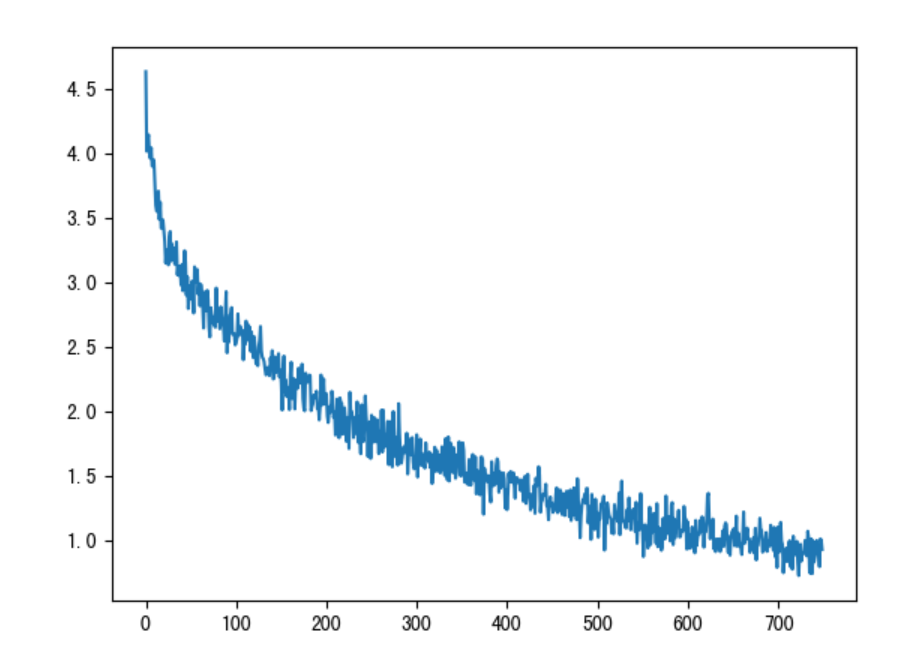
一直下降的损失曲线, 说明模型正在收敛, 能够从数据中找到一些规律应用于数据。

5.构建模型评估函数并测试

（1）构建模型评估函数

# 模型评估代码与模型预测代码类似，需要注意使用with torch.no_grad()
# 模型预测时，第一个时间步使用SOS_token作为输入 后续时间步采用预测值作为输入，也就是自回归机制
def Seq2Seq_Evaluate(x, my_encoderrnn, my_attndecoderrnn):with torch.no_grad():# 1 编码：一次性的送数据encode_hidden = my_encoderrnn.inithidden()encode_output, encode_hidden = my_encoderrnn(x, encode_hidden)# 2 解码参数准备# 解码参数1 固定长度中间语义张量cencoder_outputs_c = torch.zeros(MAX_LENGTH, my_encoderrnn.hidden_size, device=device)x_len = x.shape[1]for idx in range(x_len):encoder_outputs_c[idx] = encode_output[0, idx]# 解码参数2 最后1个隐藏层的输出 作为 解码器的第1个时间步隐藏层输入decode_hidden = encode_hidden# 解码参数3 解码器第一个时间步起始符input_y = torch.tensor([[SOS_token]], device=device)# 3 自回归方式解码# 初始化预测的词汇列表decoded_words = []# 初始化attention张量decoder_attentions = torch.zeros(MAX_LENGTH, MAX_LENGTH)for idx in range(MAX_LENGTH): # note:MAX_LENGTH=10output_y, decode_hidden, attn_weights = my_attndecoderrnn(input_y, decode_hidden, encoder_outputs_c)# 预测值作为为下一次时间步的输入值topv, topi = output_y.topk(1)decoder_attentions[idx] = attn_weights# 如果输出值是终止符，则循环停止if topi.squeeze().item() == EOS_token:decoded_words.append('<EOS>')breakelse:decoded_words.append(french_index2word[topi.item()])# 将本次预测的索引赋值给 input_y，进行下一个时间步预测input_y = topi.detach()# 返回结果decoded_words， 注意力张量权重分布表(把没有用到的部分切掉)return decoded_words, decoder_attentions[:idx + 1]

（2）模型评估函数调用

# 加载模型
PATH1 = './gpumodel/my_encoderrnn.pth'
PATH2 = './gpumodel/my_attndecoderrnn.pth'
def dm_test_Seq2Seq_Evaluate():# 实例化dataset对象mypairsdataset = MyPairsDataset(my_pairs)# 实例化dataloadermydataloader = DataLoader(dataset=mypairsdataset, batch_size=1, shuffle=True)# 实例化模型input_size = english_word_nhidden_size = 256  # 观察结果数据 可使用8my_encoderrnn = EncoderRNN(input_size, hidden_size)# my_encoderrnn.load_state_dict(torch.load(PATH1))my_encoderrnn.load_state_dict(torch.load(PATH1, map_location=lambda storage, loc: storage), False)print('my_encoderrnn模型结构--->', my_encoderrnn)# 实例化模型input_size = french_word_nhidden_size = 256  # 观察结果数据 可使用8my_attndecoderrnn = AttnDecoderRNN(input_size, hidden_size)# my_attndecoderrnn.load_state_dict(torch.load(PATH2))my_attndecoderrnn.load_state_dict(torch.load(PATH2, map_location=lambda storage, loc: storage), False)print('my_decoderrnn模型结构--->', my_attndecoderrnn)my_samplepairs = [['i m impressed with your french .', 'je suis impressionne par votre francais .'],['i m more than a friend .', 'je suis plus qu une amie .'],['she is beautiful like her mother .', 'elle est belle comme sa mere .']]print('my_samplepairs--->', len(my_samplepairs))for index, pair in enumerate(my_samplepairs):x = pair[0]y = pair[1]# 样本x 文本数值化tmpx = [english_word2index[word] for word in x.split(' ')]tmpx.append(EOS_token)tensor_x = torch.tensor(tmpx, dtype=torch.long, device=device).view(1, -1)# 模型预测decoded_words, attentions = Seq2Seq_Evaluate(tensor_x, my_encoderrnn, my_attndecoderrnn)# print('decoded_words->', decoded_words)output_sentence = ' '.join(decoded_words)print('\n')print('>', x)print('=', y)print('<', output_sentence)

运行结果：

> i m impressed with your french .
= je suis impressionne par votre francais .
< je suis impressionnee par votre francais . <EOS>> i m more than a friend .
= je suis plus qu une amie .
< je suis plus qu une amie . <EOS>> she is beautiful like her mother .
= elle est belle comme sa mere .
< elle est sa sa mere . <EOS>> you re winning aren t you ?
= vous gagnez n est ce pas ?
< tu restez n est ce pas ? <EOS>> he is angry with you .
= il est en colere apres toi .
< il est en colere apres toi . <EOS>> you re very timid .
= vous etes tres craintifs .
< tu es tres craintive . <EOS>

（3） Attention张量制图

def dm_test_Attention():# 实例化dataset对象mypairsdataset = MyPairsDataset(my_pairs)# 实例化dataloadermydataloader = DataLoader(dataset=mypairsdataset, batch_size=1, shuffle=True)# 实例化模型input_size = english_word_nhidden_size = 256  # 观察结果数据 可使用8my_encoderrnn = EncoderRNN(input_size, hidden_size)# my_encoderrnn.load_state_dict(torch.load(PATH1))my_encoderrnn.load_state_dict(torch.load(PATH1, map_location=lambda storage, loc: storage), False)# 实例化模型input_size = french_word_nhidden_size = 256  # 观察结果数据 可使用8my_attndecoderrnn = AttnDecoderRNN(input_size, hidden_size)# my_attndecoderrnn.load_state_dict(torch.load(PATH2))my_attndecoderrnn.load_state_dict(torch.load(PATH2, map_location=lambda storage, loc: storage), False)sentence = "we re both teachers ."# 样本x 文本数值化tmpx = [english_word2index[word] for word in sentence.split(' ')]tmpx.append(EOS_token)tensor_x = torch.tensor(tmpx, dtype=torch.long, device=device).view(1, -1)# 模型预测decoded_words, attentions = Seq2Seq_Evaluate(tensor_x, my_encoderrnn, my_attndecoderrnn)print('decoded_words->', decoded_words)# print('\n')# print('英文', sentence)# print('法文', output_sentence)plt.matshow(attentions.numpy()) # 以矩阵列表的形式 显示# 保存图像plt.savefig("./s2s_attn.png")plt.show()print('attentions.numpy()--->\n', attentions.numpy())print('attentions.size--->', attentions.size())

运行结果：

decoded_words-> ['nous', 'sommes', 'toutes', 'deux', 'enseignantes', '.', '<EOS>']

Attention可视化:

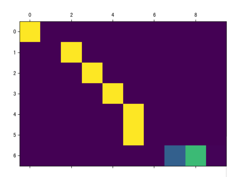
Attention图像的纵坐标代表输入的源语言各个词汇对应的索引：

0-6分别对应[“we”, “re”, “both”, “teachers”, “.”, “”], 纵坐标代表生成的目标语言各个词汇对应的索引, 0-7代表[‘nous’, ‘sommes’, ‘toutes’, ‘deux’, ‘enseignantes’, ‘.’, ‘’], 图中浅色小方块(颜色越浅说明影响越大)代表词汇之间的影响关系, 比如源语言的第1个词汇对生成目标语言的第1个词汇影响最大, 源语言的第4，5个词对生成目标语言的第5个词会影响最大。

通过这样的可视化图像, 我们可以知道Attention的效果好坏, 进而衡量我们训练模型的可用性。

今日分享到此结束。