一、Advanced 2D plots

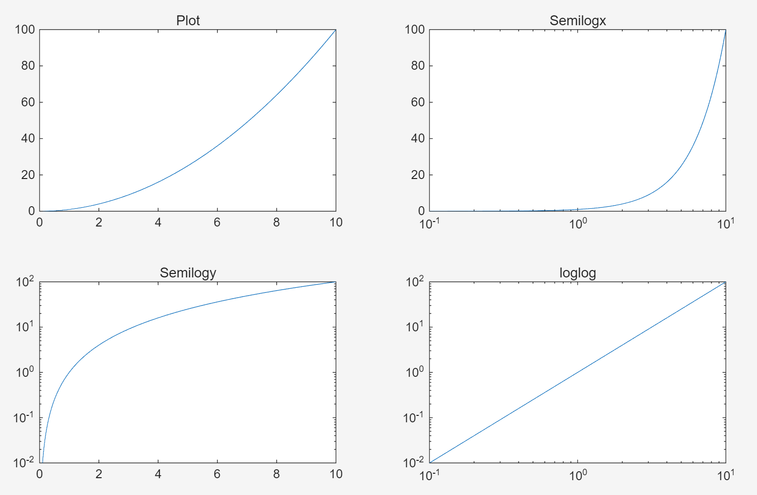
1. Logarithm Plots

x = logspace(-1,1,1000); 
% 从-1到1生成等间隔的1000个点
y = x .^ 2;
subplot(2,2,1);
plot(x,y);
title('Plot');
subplot(2,2,2);
semilogx(x,y);
title('Semilogx');
subplot(2,2,3);
semilogy(x,y);
title('Semilogy');
subplot(2,2,4);
loglog(x,y);
title('loglog');
% set(gca,'XGrid','on')

semilogx(x,y); 对 x 轴取对数
semilogy(x,y); 对 y 轴取对数
loglog(x,y); 对 x 轴和 y 轴都取对数

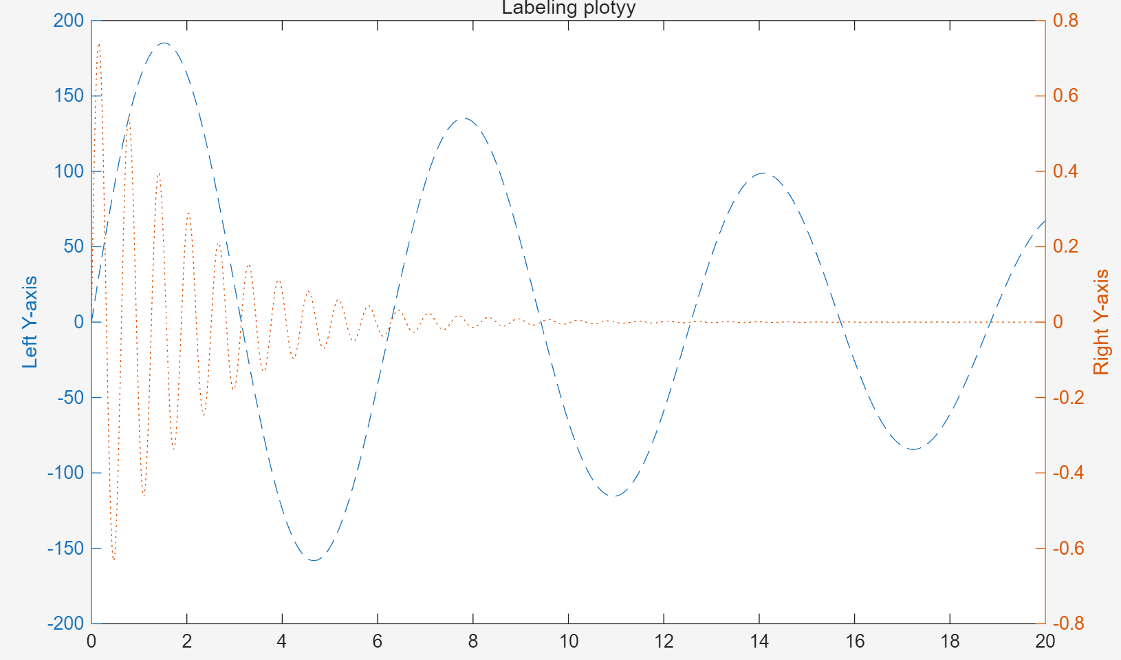
2. Plotyy()

x = 0 : 0.01 : 20;
y1 = 200 * exp(-0.05*x) .* sin(x);
y2 = 0.8 * exp(-0.5*x) .* sin(10*x);
[AX,H1,H2] = plotyy(x,y1,x,y2);
set(get(AX(1),'Ylabel'),'String','Left Y-axis');
set(get(AX(2),'Ylabel'),'String','Right Y-axis');
title('Labeling plotyy');
set(H1,'LineStyle','--');
set(H2,'LineStyle',':');

[AX,H1,H2] = plotyy(x,y1,x,y2);

共用 x 轴，AX返回包含两个坐标轴句柄的数组[AX(1),AX(2)],分别对应左侧 Y 轴和右侧 Y 轴

H1、H2:分别返回左侧 (y1) 和右侧 (y2) 数据曲线的句柄
set(get(AX(1),'Ylabel'),'String','Left Y-axis');

获得左边的y轴坐标句柄，将标签改为Left Y-axis
set(get(AX(2),'Ylabel'),'String','Right Y-axis');

获得右边的y轴坐标句柄，将标签改为Right Y-axis

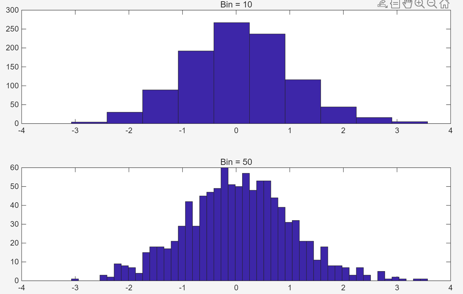
3.Histogram

y = randn(1,1000);
subplot(2,1,1);
hist(y,10);
title('Bin = 10');
subplot(2,1,2);
hist(y,50);
title('Bin = 50');

hist 将y中所有元素按照bin的个数进行分组，bin等于10，则所有y值，被分为10组，并在图上用10个等宽度的矩形来表示这10个分组，每个矩阵的高度就表示bin中的元素数量，每个bin中元素的个数是所有y中的元素，依据x轴坐标有序划入上介于每个bin横坐标的最大值和最小值间的y元素数量。

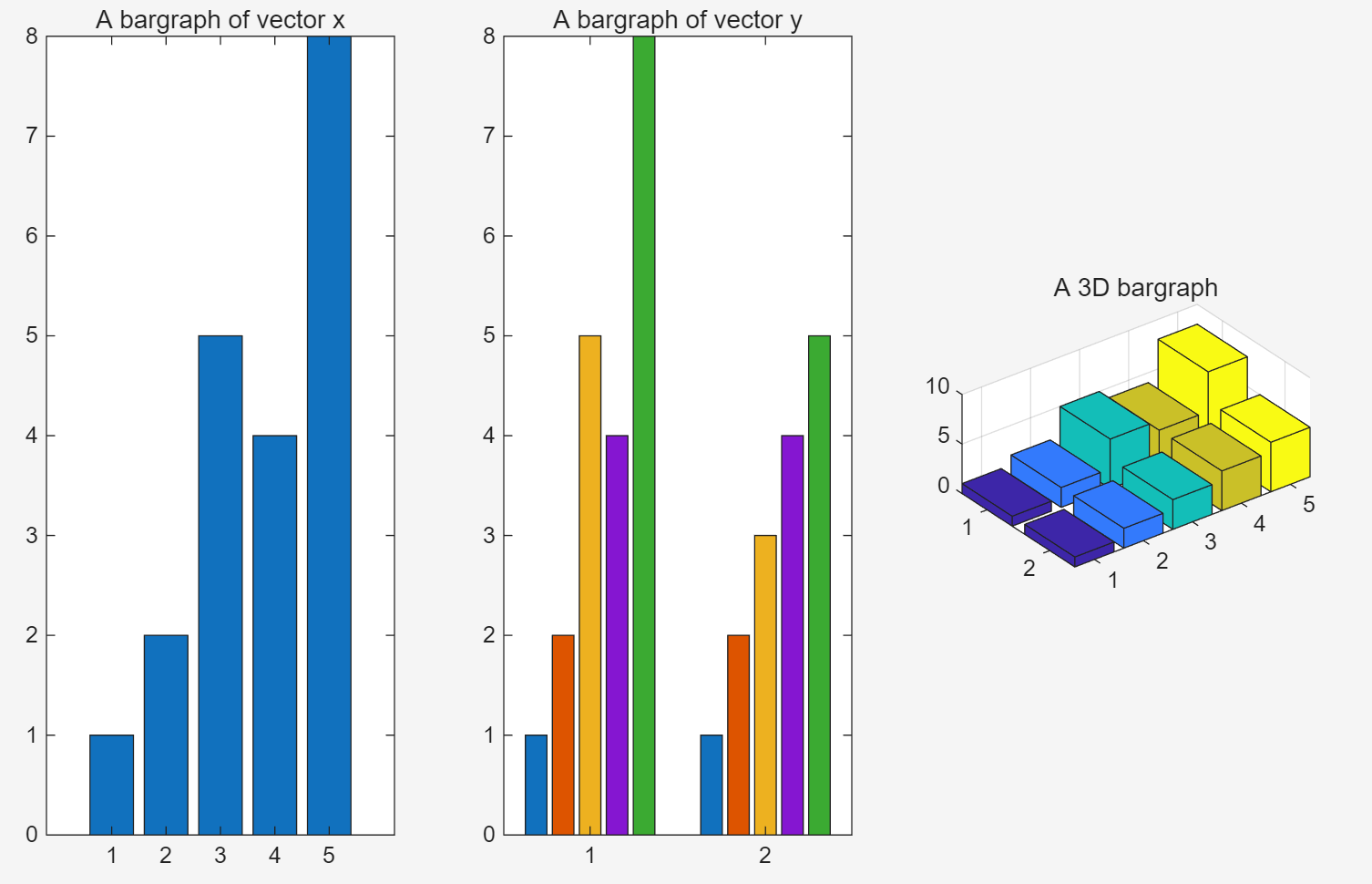
4.Bar Charts

x = [1 2 5 4 8];
y = [x;1:5];
subplot(1,3,1);bar(x);title('A bargraph of vector x');
subplot(1,3,2);bar(y);title('A bargraph of vector y');
subplot(1,3,3);bar3(y);title('A 3D bargraph');

3D图形中宽方向表示组别，长方向表示组内元素，高方向表示元素大小

第一个图条形图，第二个将两个组别分开统计做了两个条形图

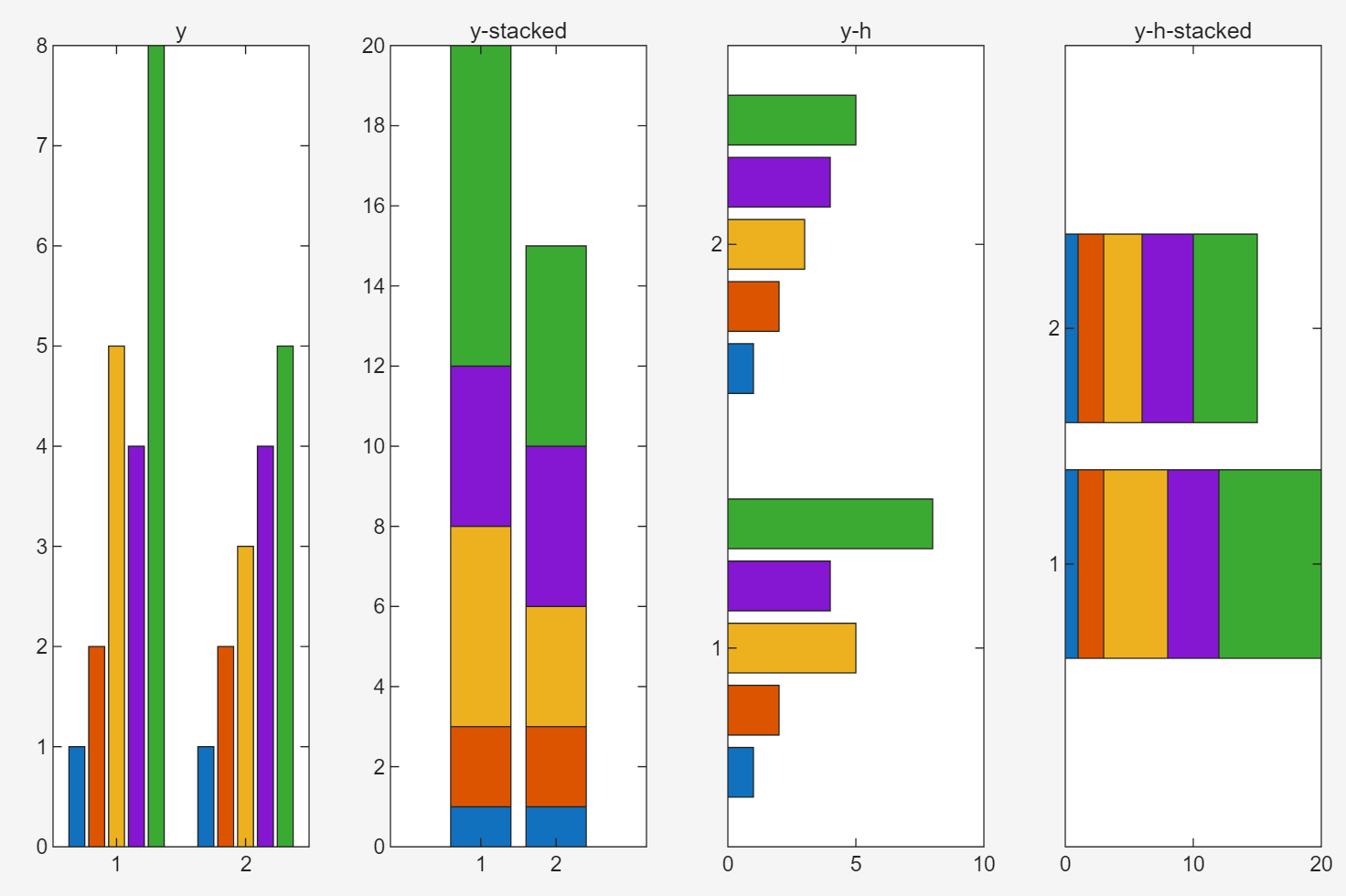
5. Stacked and Horizontal Bar Charts

x = [1 2 5 4 8];
y = [x;1:5];
subplot(1,4,1);
bar(y);
title('y');
subplot(1,4,2);
bar(y,'stacked');
title('y-stacked');
subplot(1,4,3);
barh(y);
title('y-h');
subplot(1,4,4);
barh(y,'stacked');
title('y-h-stacked');

bar后面加h，变成barh表示在生成的条状图平行与水平面（horizontal），

' stacked ' 表示在特定方向上的条状图堆叠

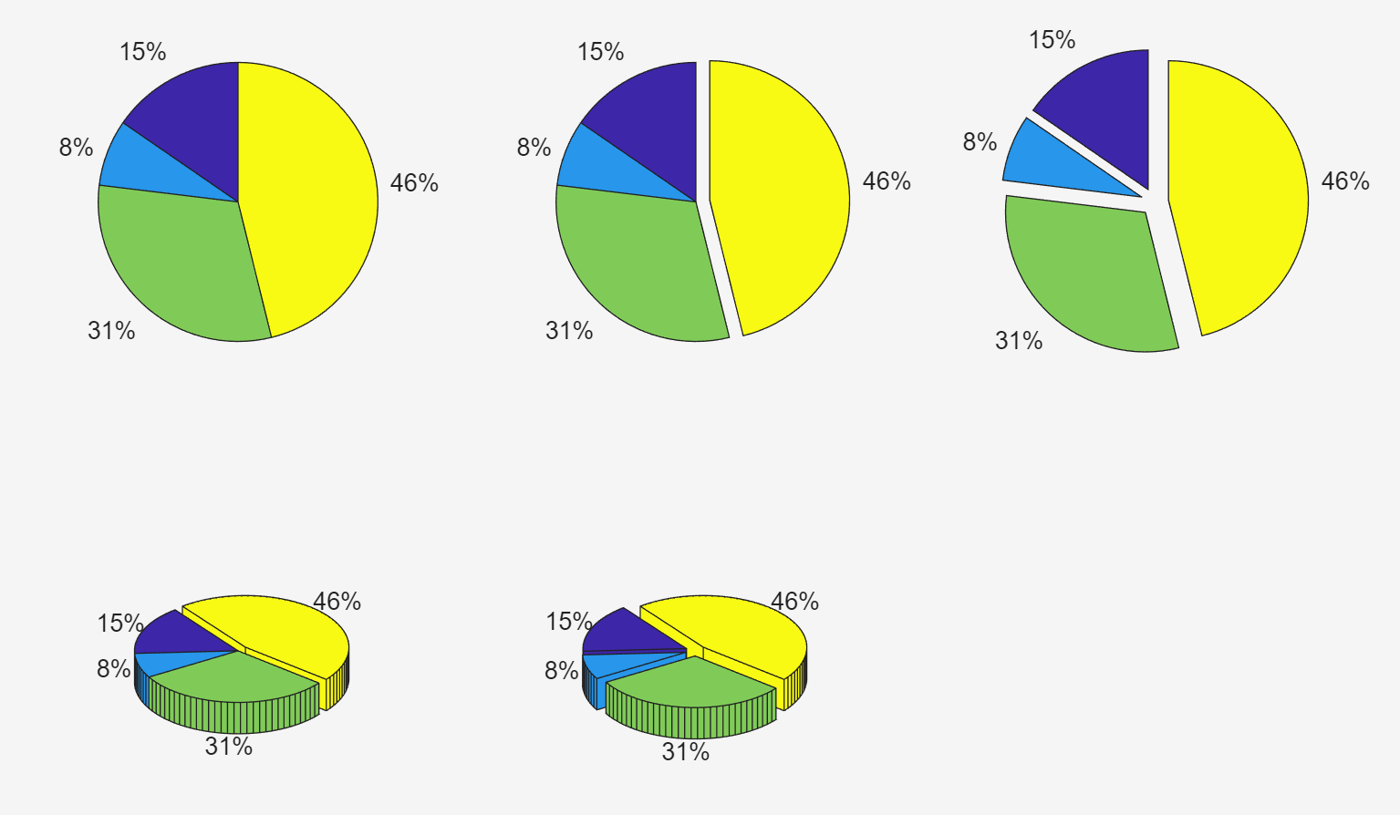
6. Pie Charts

a = [10 5 20 30];
subplot(2,3,1); pie(a);
subplot(2,3,2); pie(a,[0,0,0,1]);
subplot(2,3,3); pie(a,[1,1,1,1]);
subplot(2,3,4); pie3(a,[0,0,0,1]);
subplot(2,3,5); pie3(a,[1,1,1,1]);

pie(a); 饼图，画扇形图；pie3（）后面加个3代表3D图形
subplot(2,3,2); pie(a,[0,0,0,1]);

数组[0，0，0，1]代表扇形分片是否割裂开，0代表不割裂，1代表割裂

7.Polar Char

theta = linspace（0，2*pi）
生成一个从 0 到 2 的等间距角度数组 theta ，默认包含 100 个点。

x = 1:100;theta = x/10;r = log10(x);
subplot(2,3,1);polarplot(theta,r);
theta = linspace(0,2*pi);r = cos(4*theta);
subplot(2,3,2);polarplot(theta,r);
theta = linspace(0,2*pi,6);r = ones(1,length(theta));
subplot(2,3,3);polarplot(theta,r);
theta = linspace(0,2*pi,7);r = ones(1,length(theta));
subplot(2,3,4);polarplot(theta,r);
theta = linspace(0,2*pi);r = 1- sin(theta);
subplot(2,3,5);polarplot(theta,r);

theta = linspace(0,2*pi,6); 在0~2 $\pi$ 范围内生成 6 个间隔相等的点

r = ones(1,length(theta)); 生成 1 * length（theta）大小的矩阵，且值全为 1

polarplot(theta,r); theta 极坐标的角度，r 极坐标的半径

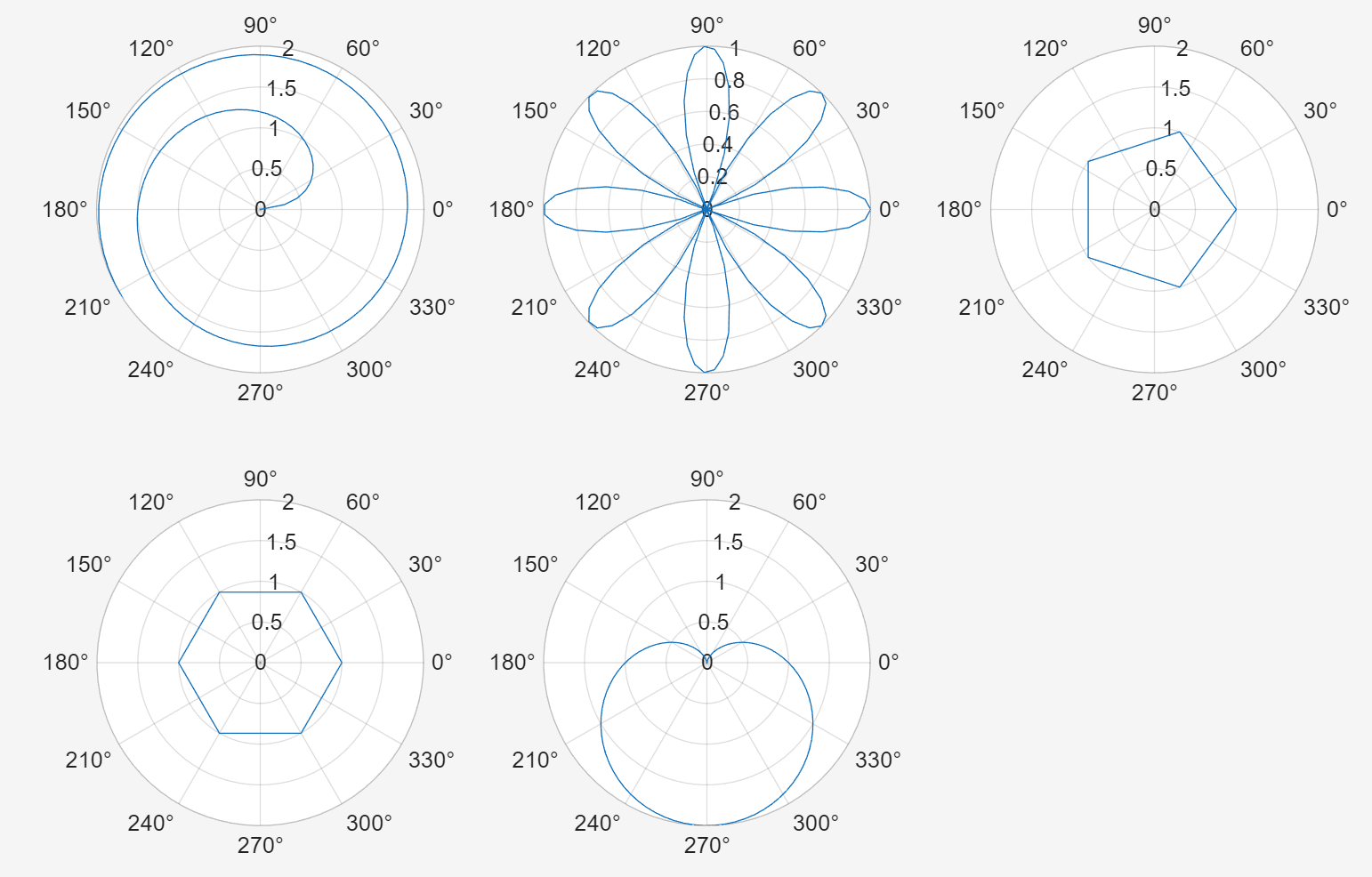
好看b（￣▽￣）d　！！

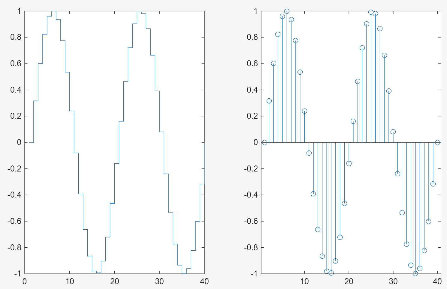
8.Stairs and Stem Charts

x = linspace(0,4*pi,40); y = sin(x);
subplot(1,2,1);stairs(y);
subplot(1,2,2);stem(y);

函数Stairs()用折线将取的点连起来，函数stem()是做出针状图

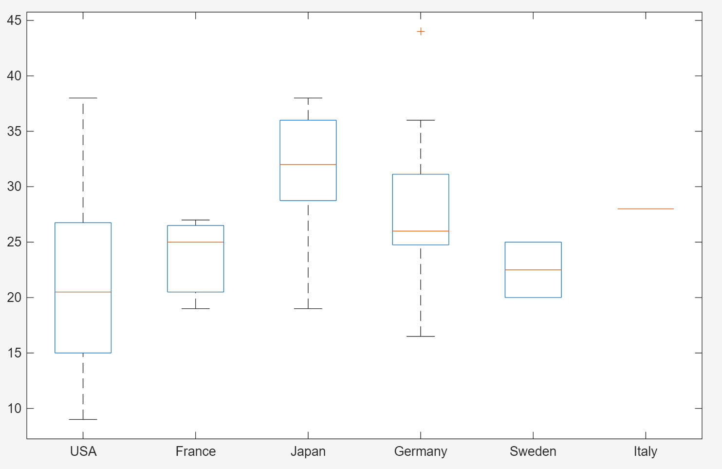
9.Boxplot and Error Bar

load carsmall.mat
boxplot(MPG,Origin);

① 使用 carsmall.mat 数据集绘制 MPG（每加仑英里数，Miles Per Gallon）

② 按 Origin（汽车原产国）分组对 MPG（每加仑英里数，Miles Per Gallon) 分类的箱线图

③ 函数boxplot（），boxplot（MPG，Origin）会根据Origin的分组，为每组MPG数据绘制一个箱线图。箱线图显示：中位数、上下四分位数、离群值（圆圈表示）等统计信息。

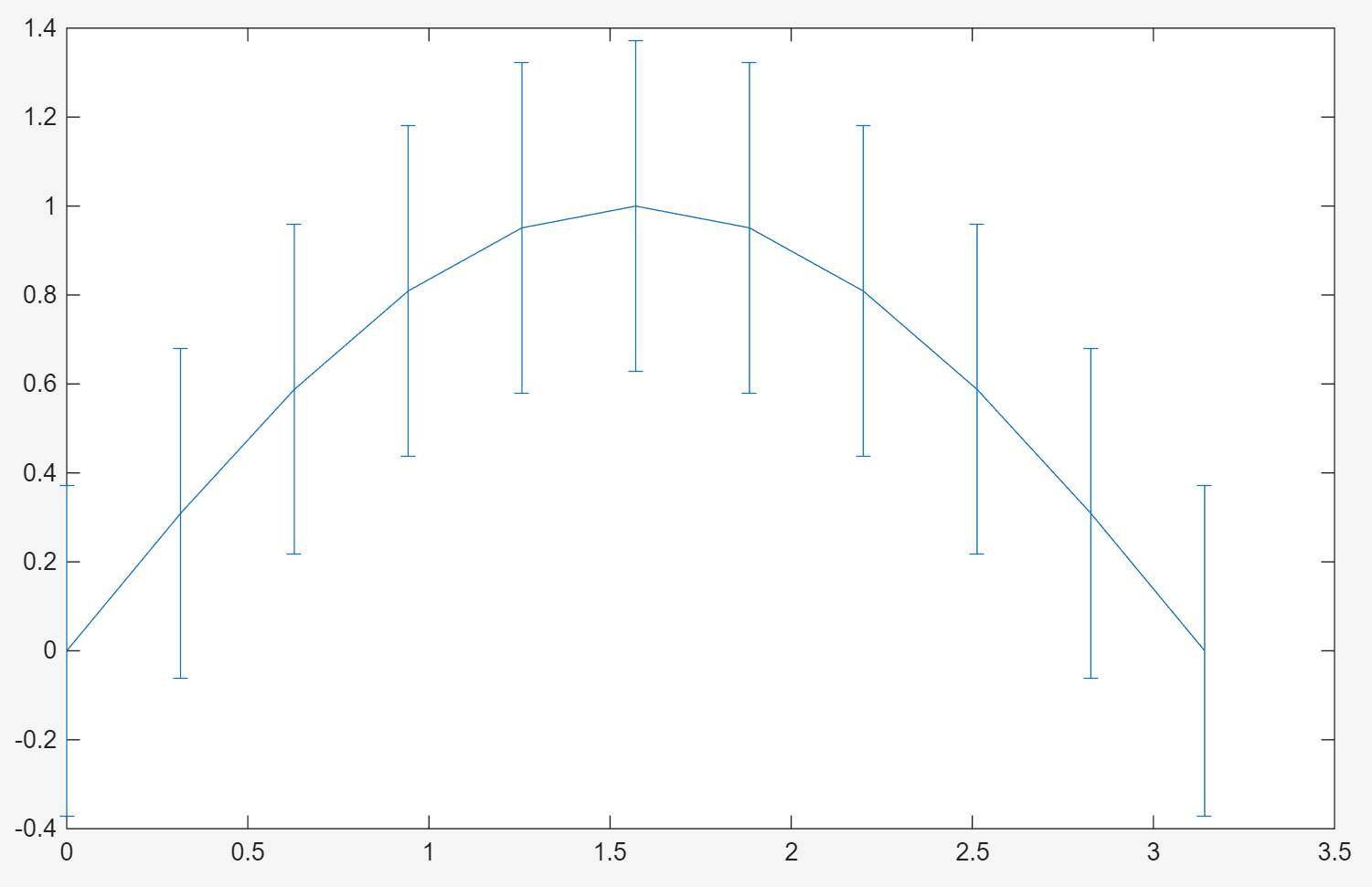
x = 0: pi/10:pi;
y =  sin(x);
e = std(y) * ones(size(x));
errorbar(x,y,e);

使用 std(y) (y的标准差）作为所有数据点的固定误差值，通过 e = std(y) * ones(size(x)); 复制为与x等长的向量。这种处理方式表示所有数据点的误差相同。误差条会以垂直线段显示在每个数据点周围，线段长度 = e 的值，即 std（y）。

10.fill（）

t = (1:2:15)' * pi/8;
x = sin(t);
y = cos(t);
fill(x,y,'r');
axis square off;
text(0,0,'STOP','Color','w','FontSize',80, ...'FontWeight','bold','HorizontalAlignment','center');

t = (1:2:15)' * pi/8; 生成等差顺序的角度序列， $\frac{\pi}{8 }$ ， $\frac{3\pi}{8 }$ ， $\frac{5\pi}{8 }$ ， $\frac{7\pi}{8 }$ ......

x = sin(t); % 将角度转化为 x 坐标

y = cos(t); % 将角度转化为 y 坐标

fill(x,y,'r'); % 将八边形内部涂上红色

axis square off; % 关闭坐标轴的方形设定

text(0,0,'STOP','Color','w','FontSize',80, ...
'FontWeight','bold','HorizontalAlignment','center');

% 设置图形的样式 STOP 白色字体放中央，字体大小80，加粗bold，字体放置中央

二、Color Space

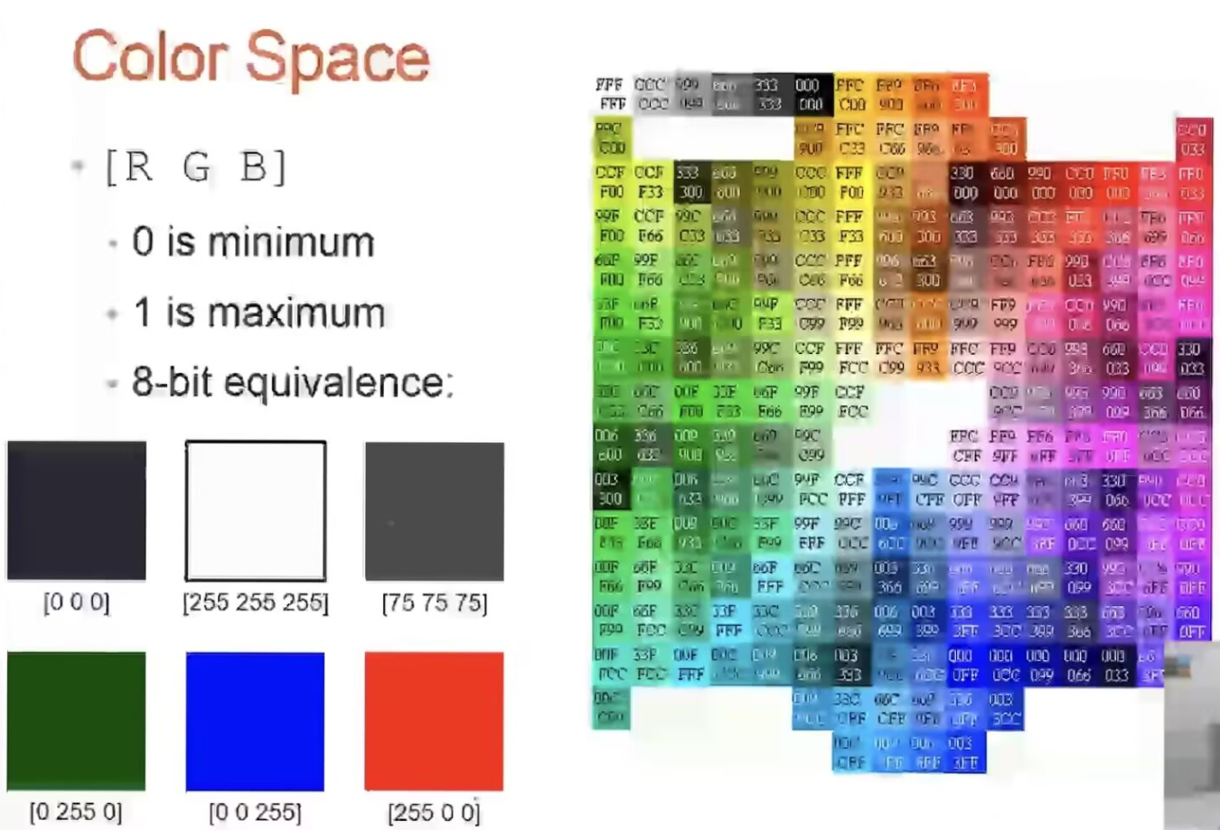
颜色有两种表达方式：

① 0 0 0 表示纯黑色，1 1 1 表示纯白色，介于 0 0 0 ~ 1 1 1 之间是灰度。

② 0 0 0 表示纯黑色，255 255 255 表示纯白色，0 255 0 表示纯绿色，0 0 255 表示纯蓝色，

255 0 0 表示纯红色

③ 三个数字分别对应 [ R G B ] 每个颜色的色度值

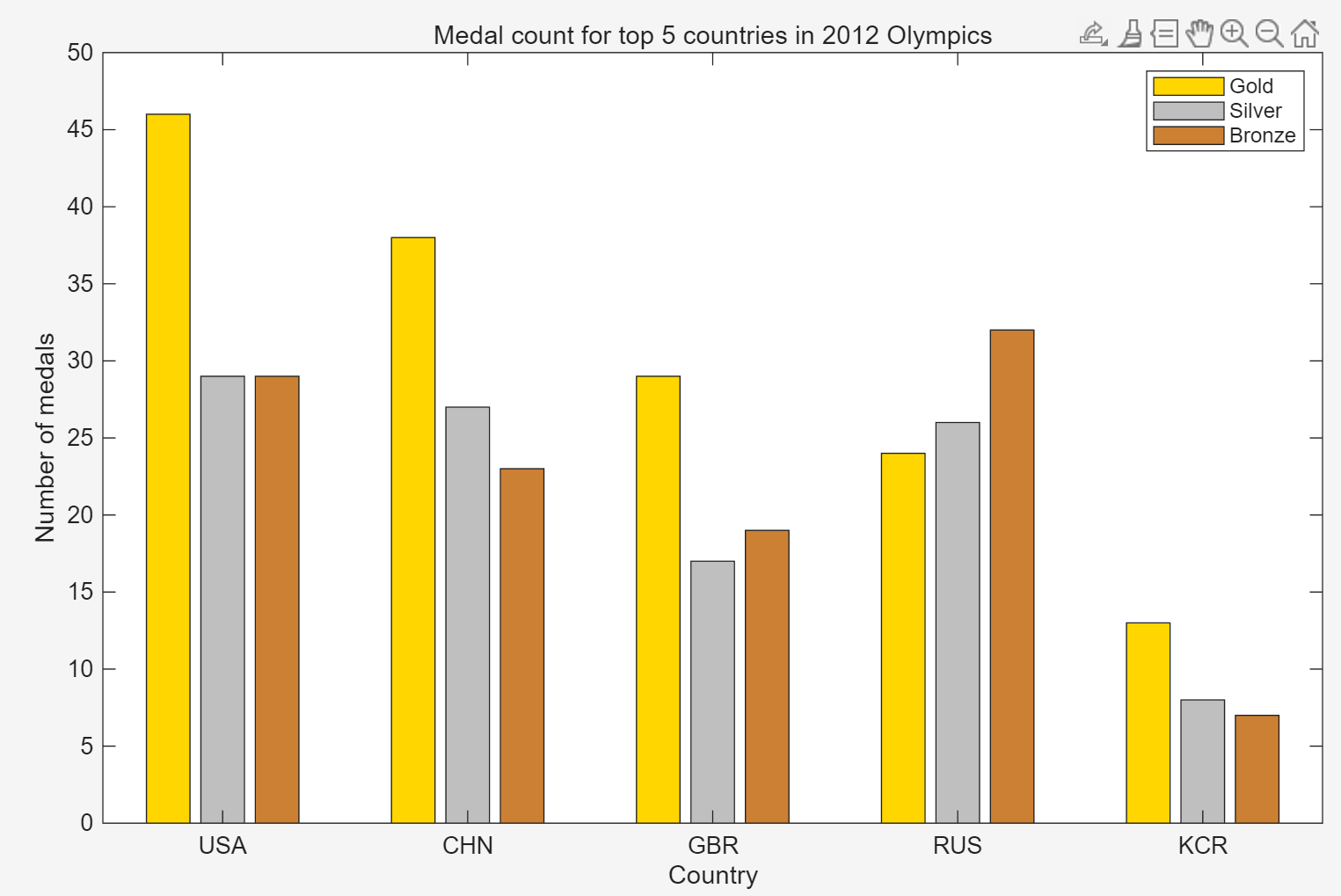
G = [46 38 29 24 13];  % 金牌数据（USA, CHN, GBR, RUS, KCR）
S = [29 27 17 26 8];   % 银牌数据
B = [29 23 19 32 7];   % 铜牌数据% 绘制堆叠条形图（每组柱子包含G/S/B三个部分）
h = bar(1:5, [G' S' B']);  % 设置X轴标签为国家名称
set(gca, 'XTickLabel', {'USA','CHN','GBR','RUS','KCR'});  % 自定义颜色（金色、银色、铜色）
set(h(1), 'FaceColor', [1 0.84 0]);  % 金色 (Gold)
set(h(2), 'FaceColor', [0.75 0.75 0.75]); % 银色 (Silver)
set(h(3), 'FaceColor', [0.8 0.5 0.2]);    % 铜色 (Bronze)% 添加标题和轴标签
title('Medal count for top 5 countries in 2012 Olympics');
xlabel('Country');
ylabel('Number of medals');% 添加图例
legend('Gold', 'Silver', 'Bronze');

set(h(1), 'FaceColor', [1 0.84 0]);

% 金色 (Gold) = 红色分量R（1）+ 绿色分量G（0.84）+ 蓝色分量（0)

% h（1）第一条柱子颜色

set(h(2), 'FaceColor', [0.75 0.75 0.75]);

% 银色 (Silver)= 红色分量R（0.75）+ 绿色分量G（0.75）+ 蓝色分量（0.75)

% h（2）第二条柱子颜色

set(h(3), 'FaceColor', [0.8 0.5 0.2]);

% 铜色 (Bronze)= 红色分量R（0.8）+ 绿色分量G（0.5）+ 蓝色分量（0.2）

% h（3）第三条柱子颜色

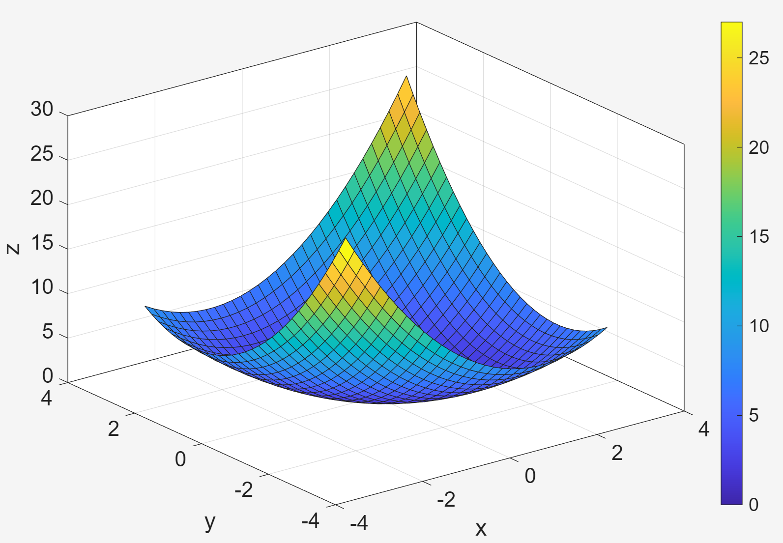
1. Visualizing Data as An Image：imagesc（）

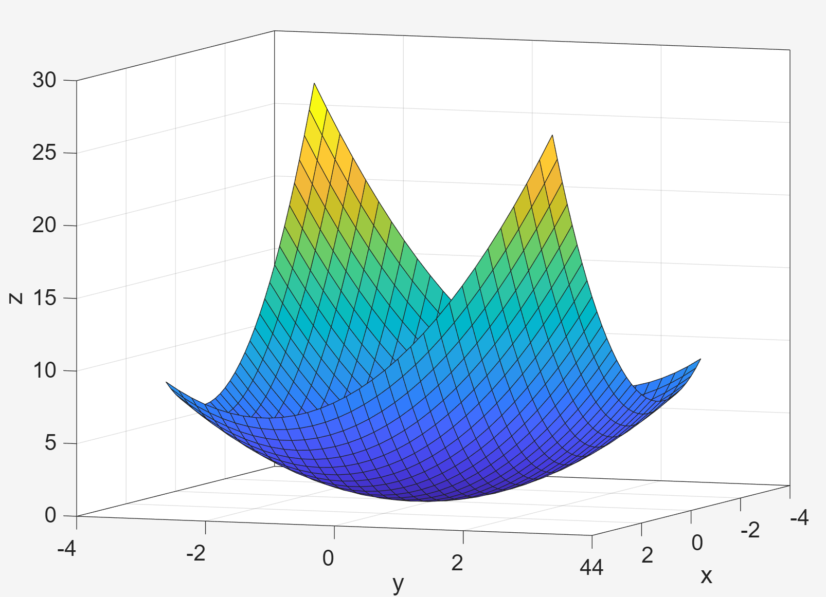
① meshgrid(x,y)的功能是：根据给定的向量 x 和 y ，生成二维网格平面上的所有坐标点组合，返回两个矩阵 x 和 y，分别表示所有点的 x 坐标和 y 坐标。

② surf（x，y，z）函数：根据给定的网格坐标（x，y）和高度值 z ，绘制三维曲面。曲面的颜色默认由 z 值决定，可通过 colormap 修改。

③ box on 命令：显示所有三个维度的边框。

[x,y] = meshgrid(-3:.2:3,-3:.2:3);
z = x.^2 + x.*y + y.^ 2;
surf(x,y,z);
box on;
set(gca,'FontSize',16);
zlabel('z');
xlim([-4 4]);
xlabel('x');
ylim([-4 4]);
ylabel('y');

2. Color Bar and Scheme

colorbar; 添加颜色条

colormap（cool）；colormap（hot）；colormap（gray）；

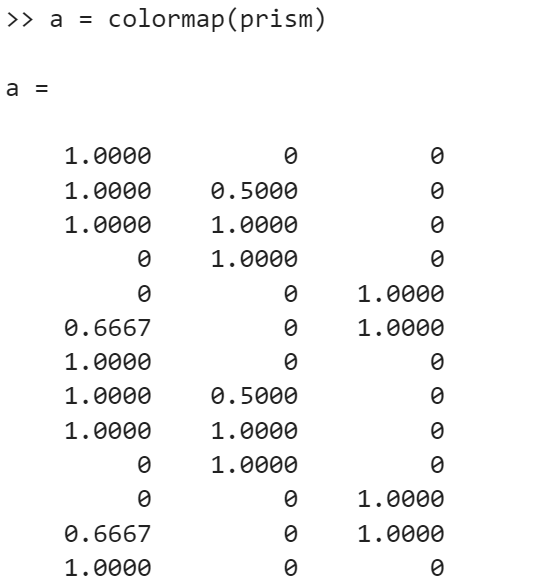
3. Built-in Colormaps

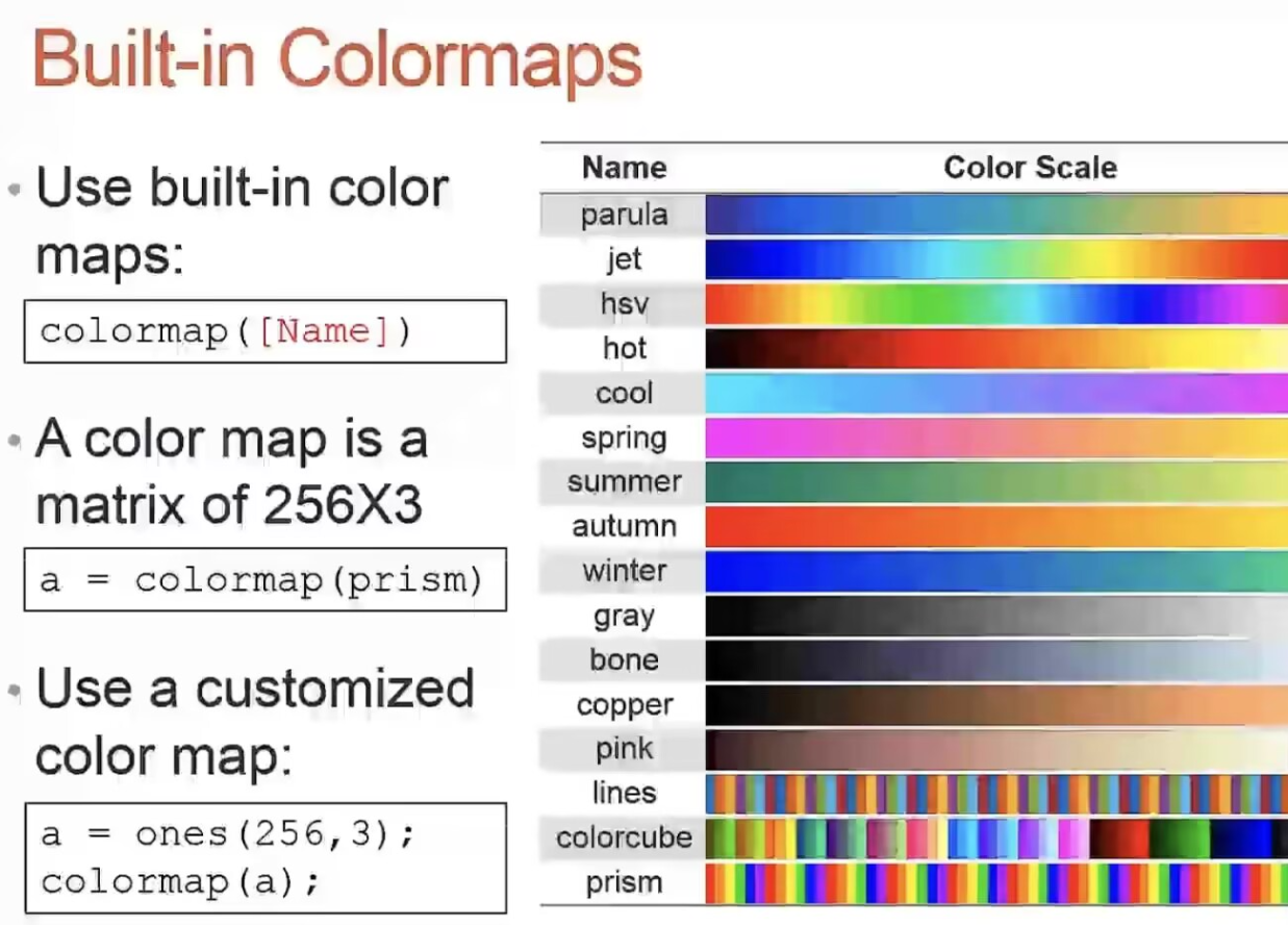
每一个colormap都是一个256*3的矩阵

4.Exercise

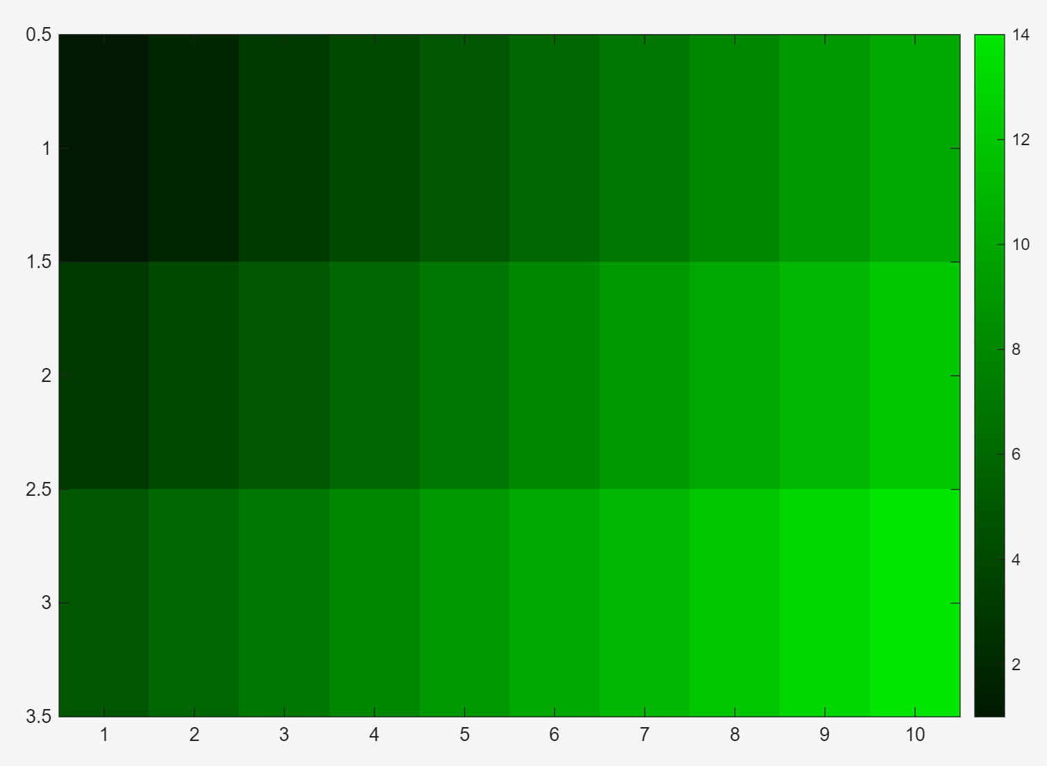
a = zeros(256,3);
a(:,1) = 0;
a(:,2) = linspace(0.1,0.9,length(a));
a(:,3) = 0;
colormap(a);
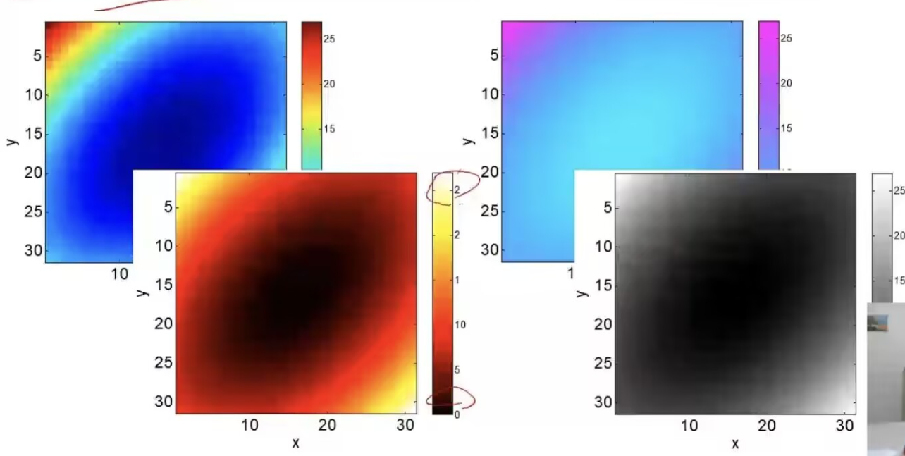
x = [1:10;3:12;5:14];
imagesc(x);
colorbar;

① Colormap是 256 * 3 的矩阵，前四行定义 a 矩阵存储绿色 colormap 的256 * 3 的矩阵

因为是绿色系，所以第一列红色分量R全为0，且第三列蓝色分量B也全为0，

第二列绿色分量G也就是在0~1中生成256个等间距的绿色颜色值，然后把定义的 x 数组涂上颜色

② imagesc（x）是一个用于可视化矩阵数据的函数，它会将矩阵 x 的值映射为彩色图像，并自动缩放颜色范围以适应数据。

三、3D Plots

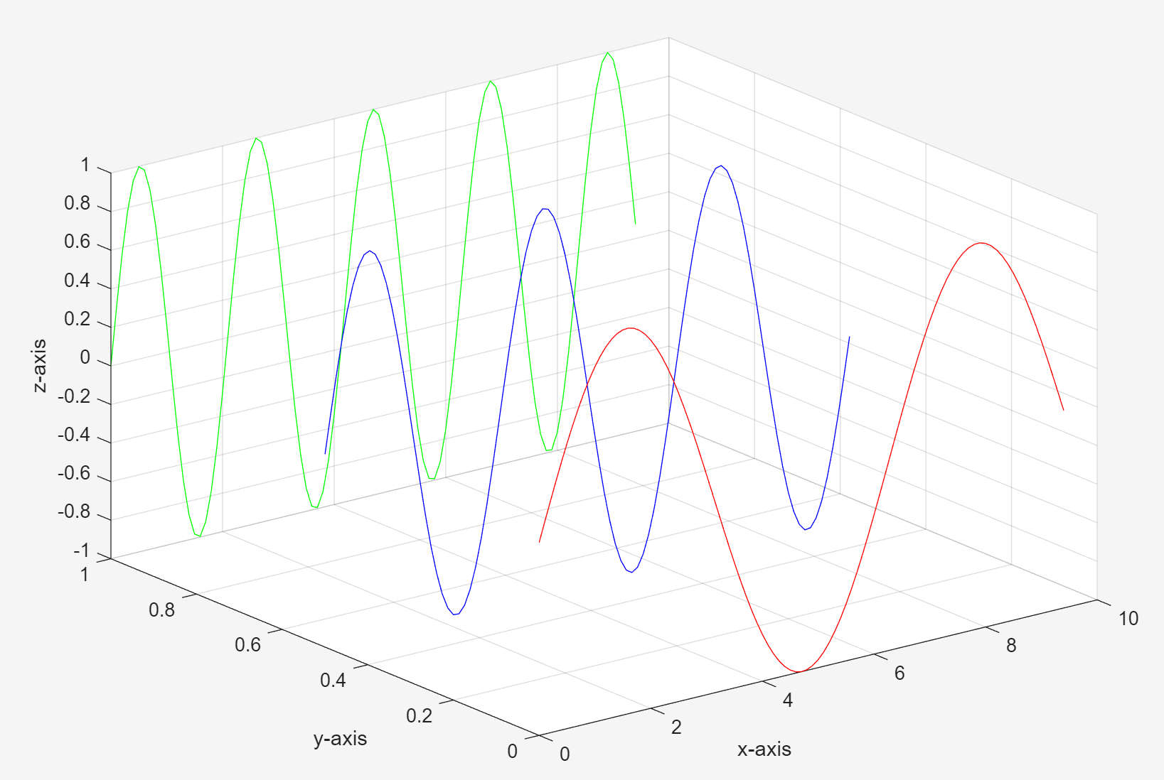
1.plot3（）

x = 0:0.1:3*pi;z1 = sin(x);z2 = sin(2*x);z3 = sin(3*x);
y1 = zeros(size(x));y3 = ones(size(x));y2 = y3 ./2;
plot3(x,y1,z1,'r',x,y2,z2,'b',x,y3,z3,'g');grid on;
xlabel('x-axis');ylabel('y-axis');zlabel('z-axis');

x = 0:0.1:3*pi;z1 = sin(x);z2 = sin(2*x);z3 = sin(3*x);

% 设置所有点的 x 坐标和 z 坐标
y1 = zeros(size(x));y3 = ones(size(x));y2 = y3 ./2;

% 设置第一条直线上所有点的y坐标都是0，第二条直线上所有点的y坐标都是0.5，第三条直线上所有点的y坐标都是1

2. More 3D Line Plots

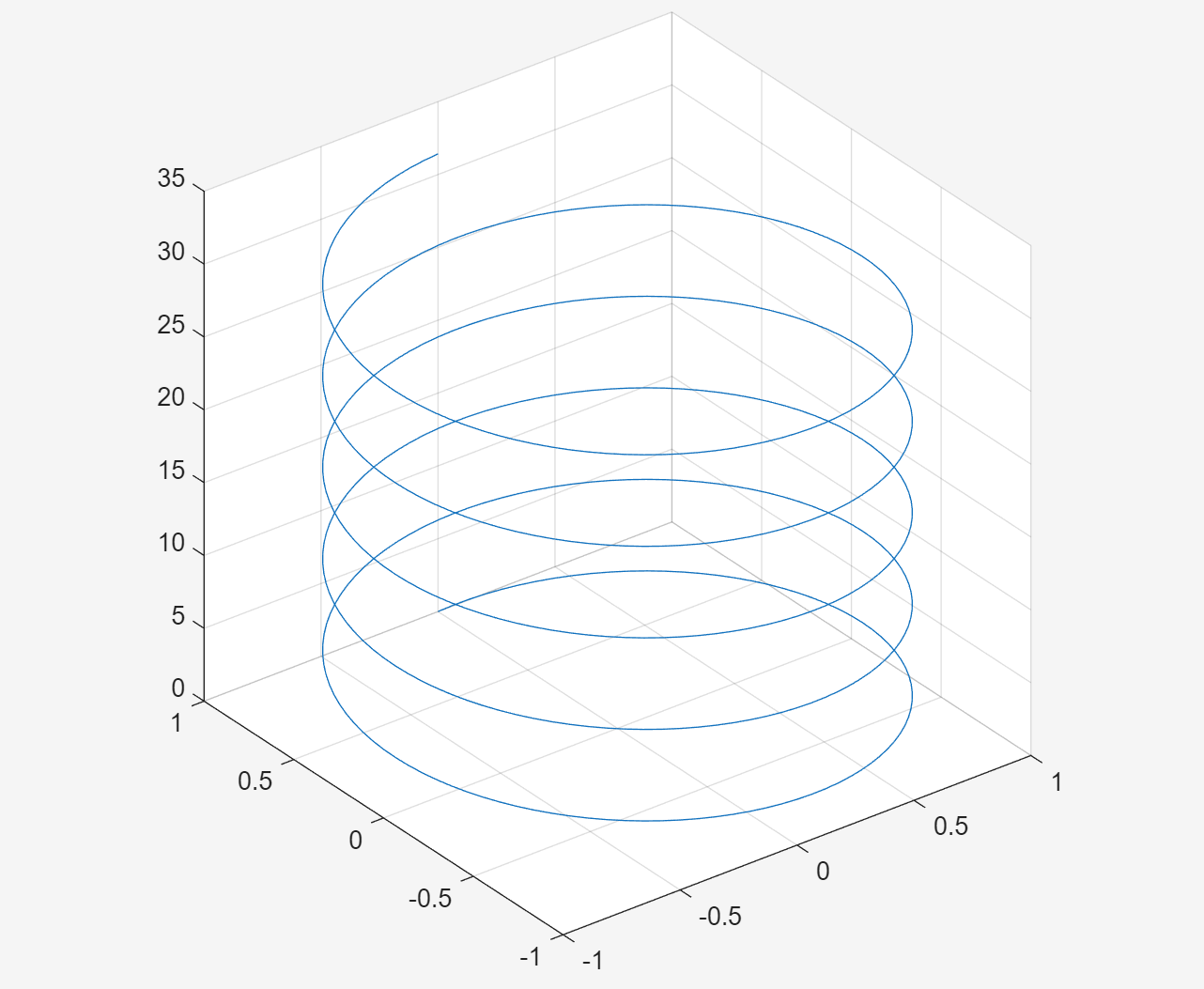
t = 0:pi/50:10*pi;
plot3(sin(t),cos(t),t);
grid on;axis square;

螺旋线：横坐标是 sin(t) 、纵坐标是 cos(t) 、高度是 t

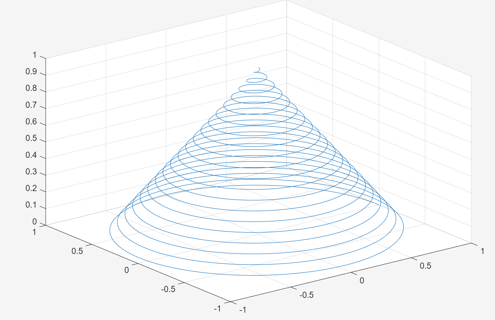
turns = 40*pi;
t = linspace(0,turns,4000);
x = cos(t) .* (turns - t) ./turns;
y = sin(t) .* (turns - t) ./turns;
z = t ./ turns;
plot3(x,y,z);grid on;

锥形螺旋线：横坐标是 cos(t) .* (turns - t) ./turns 、纵坐标是 sin(t) .* (turns - t) ./turns

高度是 t ./ turns;

3.Principles for 3D Surface Plots

meshgrid(x,y)的功能是：根据给定的向量 x 和 y ，生成二维网格平面上的所有坐标点组合，返回两个矩阵 x 和 y，分别表示所有点的 x 坐标和 y 坐标。

x = -2:1:2;
y = -2:1:2;
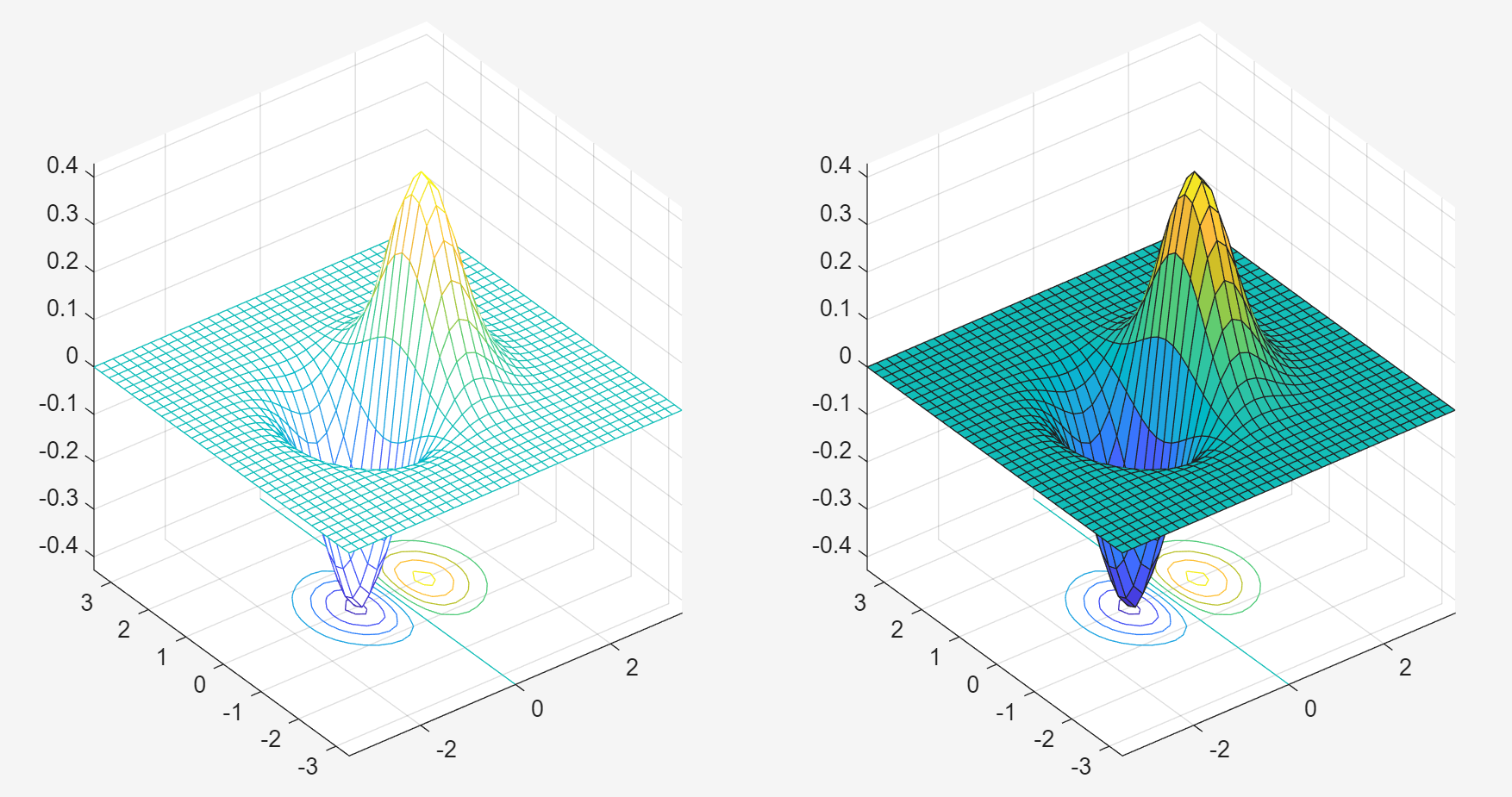
[X,Y] = meshgrid(x,y);

4.Surface Plots: mesh() and surf()

x = -3.5:0.2:3.5;
y = -3.5:0.2:3.5;
[X,Y] = meshgrid(x,y);
Z = X .* exp(-X .^2 - Y .^ 2);
subplot(1,2,1); mesh(X,Y,Z);
subplot(1,2,2); surf(X,Y,Z);

mesh(X，Y，Z) 网格曲面图：仅显示曲面的网格线（Wireframe），不填充网格面颜色。

surf(X，Y，Z) 表面曲面图：显示曲面的填充面和网格线。

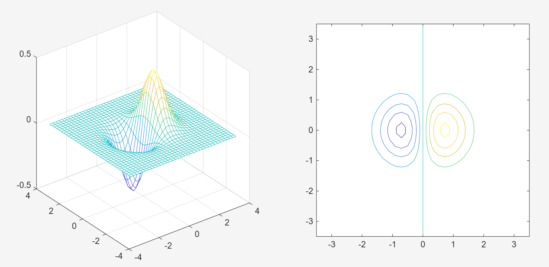
5.contour()

x = -3.5:0.2:3.5;
y = -3.5:0.2:3.5;
[X,Y] = meshgrid(x,y);
Z = X .* exp(-X .^2 - Y .^ 2);
subplot(1,2,1); mesh(X,Y,Z);
axis square;
subplot(1,2,2); contour(X,Y,Z);
axis square;

contour(X，Y，Z)是一个用于绘制二维等高线图的函数，它通过等高线来可视化三维数据 Z 的分布。将三维曲面 Z 投影到二维平面，用闭合曲线（等高线）表示相同 Z 值的区域。

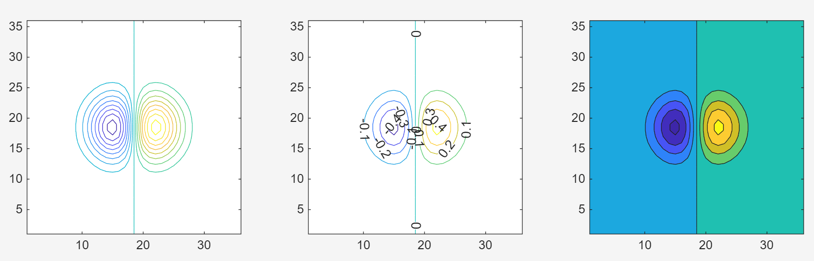
6. Various Contoyr Plots

x = -3.5:0.2:3.5;
y = -3.5:0.2:3.5;
[X,Y] = meshgrid(x,y);
Z = X .* exp(-X .^2 - Y .^ 2);
subplot(1,3,1); contour(Z,[-0.45:0.05:0.45]);axis square;
subplot(1,3,2); [C,h] = contour(Z);
clabel(C,h); axis square;
subplot(1,3,3); contourf(Z); axis square;

子图	代码	功能
1	contour(Z,[-0.45:0.05:0.45])	手动指定等高线层级（-0.45到0.45，步长0.05）
2	[C,h] = contour(Z)；clabel (C，h)；	自动分层+添加数值标签
3	contourf (Z)	填充颜色的等高线图（contour后加 f ，意思为 fill ）

7. Exercise

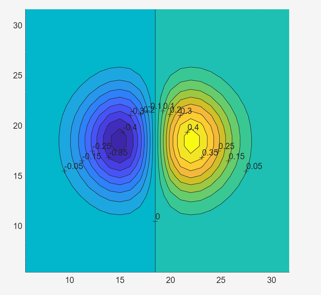
hold on
x = -3.5:0.2:3.5;
y = -3.5:0.2:3.5;
[X,Y] = meshgrid(x,y);
Z = X .* exp(-X .^2 - Y .^ 2);
clabel(contourf(Z,[-0.45:0.05:0.45])); axis square;
hold off

clabel(contourf(Z,[-0.45:0.05:0.45])); axis square;

函数clabel (C，h) 和函数contourf (Z)叠一块使用就得到含有数值的等高线图

8.meshc() and surfc()

x = -3.5 :0.2:3.5;
y = -3.35:0.2:3.5;
[X,Y] = meshgrid(x,y); Z = X.* exp(-X .^ 2 - Y .^ 2);
subplot(1,2,1); meshc(X,Y,Z);
subplot(1,2,2); surfc(X,Y,Z);

① meshc(X，Y，Z)：网格曲面 + 等高线

上方：三维网格曲面，同mesh ；底部：二维等高线投影，同contour

② sufc(X，Y，Z)：表面曲面 + 等高线

上方：三维填充曲面，同surf ；底部：二维等高线投影，同contour

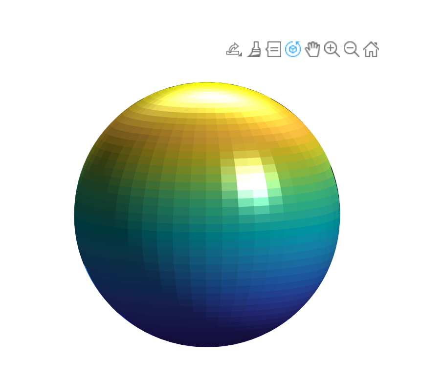
9.View Angle: view()

sphere(50);shading flat;
light('Position',[1 3 2]);
light('Position',[-3 -1 3]);
material shiny;
axis vis3d off;
set(gcf,'Color',[1 1 1]);
view(-45,20);

① sphere(50); 生成单位球面的三维坐标，默认返回50×50的网格，50 表示球面的网格细分程度，值越大越光滑。

② shading flat ；设置着色模式为平坦着色，即每个网格面单色

③ light('Position',[1 3 2])；light('Position',[-3 -1 3])；

光源三维坐标的位置，决定光照方向和阴影效果，增强立体感

④ material shiny；设置物体表面为高光材质

⑤ axis vis3d off；vis3d 保持三维比例不变形；'Color',[1 1 1]，设置图形窗口背景为白色

⑥ view(-45,20) ：方位角（Azimuth）: -45度，从正东方向逆时针旋转45度；俯仰角（Elevation) : 20 度，向上倾斜20度

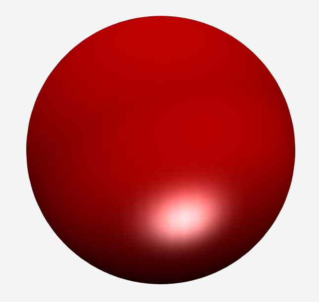
10.Ligth：light()

light（）函数用于三维图形中添加光源，通过模拟光照增强立体感和真实感。

L1 = light（'Position'，[-1，-1，-1]）； % 添加光源位置

set（L1，'Color'，'g'）； % 添加光源色彩

[X, Y, Z] = sphere(64); h = surf(X,Y,Z);
axis square vis3d off;
reds = zeros(256,3); reds(:,1) = (0:256.-1)/255;
colormap(reds); shading interp;lighting phong;
set(h,'AmbientStrength',0.75,'DiffuseStrength',0.5);
L1 = light('Position',[-1,-1,-1]);
set(L1,'Positiion',[-1,-1,1]);
set(L1,'Color','g');

① [X, Y, Z] = sphere(64); h = surf(X,Y,Z);

生成一个 64×64 网格的高精度单位球面，并绘制曲面。64是球面的网格细分程度，值越大表面越光滑；h曲面对象的句柄，用于后续属性修改。

② axis square vis3d off;

square 保持坐标轴比例一致，vis3d 在旋转时保持三维视角比例，off 隐藏坐标轴和标签。

③ reds = zeros(256,3); reds(:,1) = (0:256.-1)/255;

自定义红色渐变色图，创建一个 256×3 的零矩阵，仅填充第一列的红色通道

④ colormap(reds); 应用自定义的红色渐变色图

⑤ shading interp; 平滑着色，颜色在网格间渐变，消除网格线

lighting phong; 使用 Phong 光照，计算高光反射，效果更逼真

⑥ set(h,'AmbientStrength',0.75,'DiffuseStrength',0.5);

'AmbientStrength',0.75：增强环境光和整体亮度

'DiffuseStrength',0.5 ：减少漫反射，降低非直射光的影响

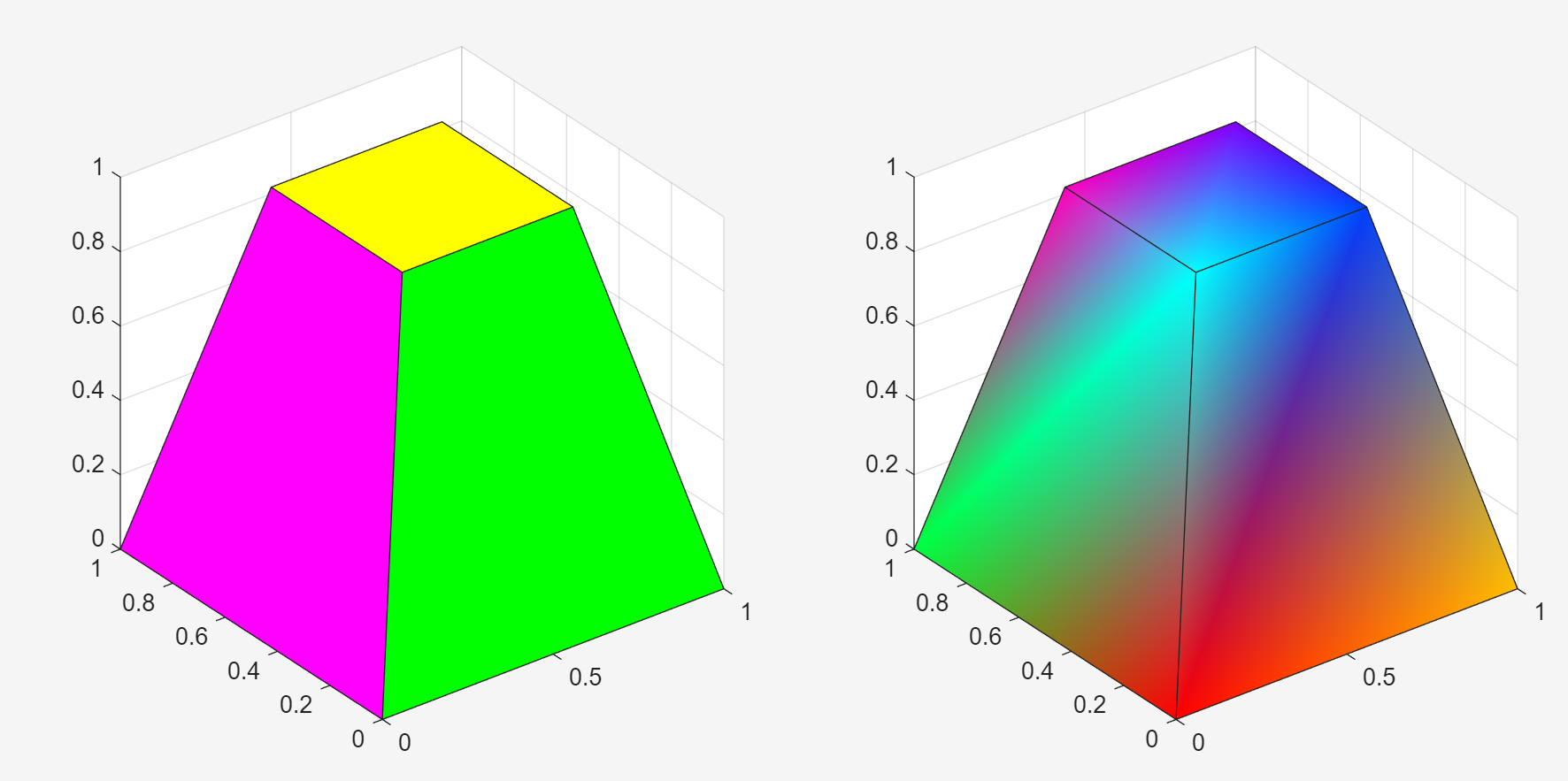
11.patch()

patch（）函数用于创建多边形面片对象，用于绘制自定义 2D/3D 形状、填充区域或构建复杂几何体。

参数	效果
' Vertices '	边缘线颜色定义所有的点
' Faces '	定义所有的面
' FaceVertexCData '	为8个顶点分配不同颜色，使用 HSV 色图的前8种颜色
' FaceColor '	每个面单色，颜色由面的第一个顶点决定

v = [0 0 0; 1 0 0; 1 1 0; 0 1 0; 0.25 0.25 1;...0.75 0.25 1;0.75 0.75 1;0.25 0.75 1];
f = [1 2 3 4; 5 6 7 8; 1 2 6 5; 2 3 7 6; 3 4 8 7 ; 4 1 5 8];
subplot(1,2,1); patch('Vertices',v,'Faces',f, ...'FaceVertexCData',hsv(6),'FaceColor','flat');
view(3); axis square tight; grid on;
subplot(1,2,2); patch('Vertices',v,'Faces',f,...'FaceVertexCData',hsv(8),'FaceColor','interp');
view(3); axis square tight; grid on;

view（3）用于设置三维图形视角的函数，根据当前坐标区的视角切换到默认的三维视图，默认方位角 -37.5°，默认俯仰角 30°