一、准备工作
电脑发出数据的波形图绘制在我的另一篇博客有详细介绍:
根据Wireshark捕获数据包时间和长度绘制电脑发射信号波形-CSDN博客
路由器发送给电脑数据的波形图绘制也在我的另一篇博客有详细介绍:
根据Wireshark捕获数据包时间和长度绘制路由器发送给电脑数据的信号波形-CSDN博客
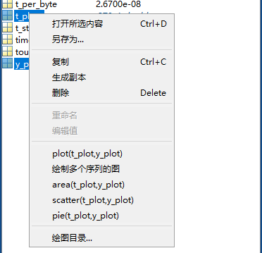
这里额外介绍了下怎么便捷保存MATLAB变量,可以用来保存绘制的电脑发射信号波形数据和路由器发射信号波形数据:
MATLAB变量便捷存储方法-CSDN博客
二、比较波形绘制
本篇文章把两个波形图绘制在一起,进行比较。程序:
%zhouzhichao
%2025年8月20日
%观察路由器、电脑互相发送的信号
clc
close all
clear
load("D:\无线通信网络认知\通信学报\5G信号\Wireshark波形绘制\direction_192_168_1_103.mat")
y_plot_1 = y_plot;
t_plot_1 = t_plot;
load("D:\无线通信网络认知\通信学报\5G信号\Wireshark波形绘制\source_192_168_1_103.mat")
y_plot_2 = y_plot;
t_plot_2 = t_plot;%% 绘图
figure;
stairs(t_plot_1, y_plot_1, 'LineWidth', 1.5);
hold on
y_plot_2=y_plot_2+1;
stairs(t_plot_2, y_plot_2, 'LineWidth', 1.5);ylim([-0.2 2.2]);
xlabel('Time (s)');
ylabel('Signal Wave');
title('Waveform from Wireshark Packets');
grid on;set(gca, 'FontName', 'Times New Roman')
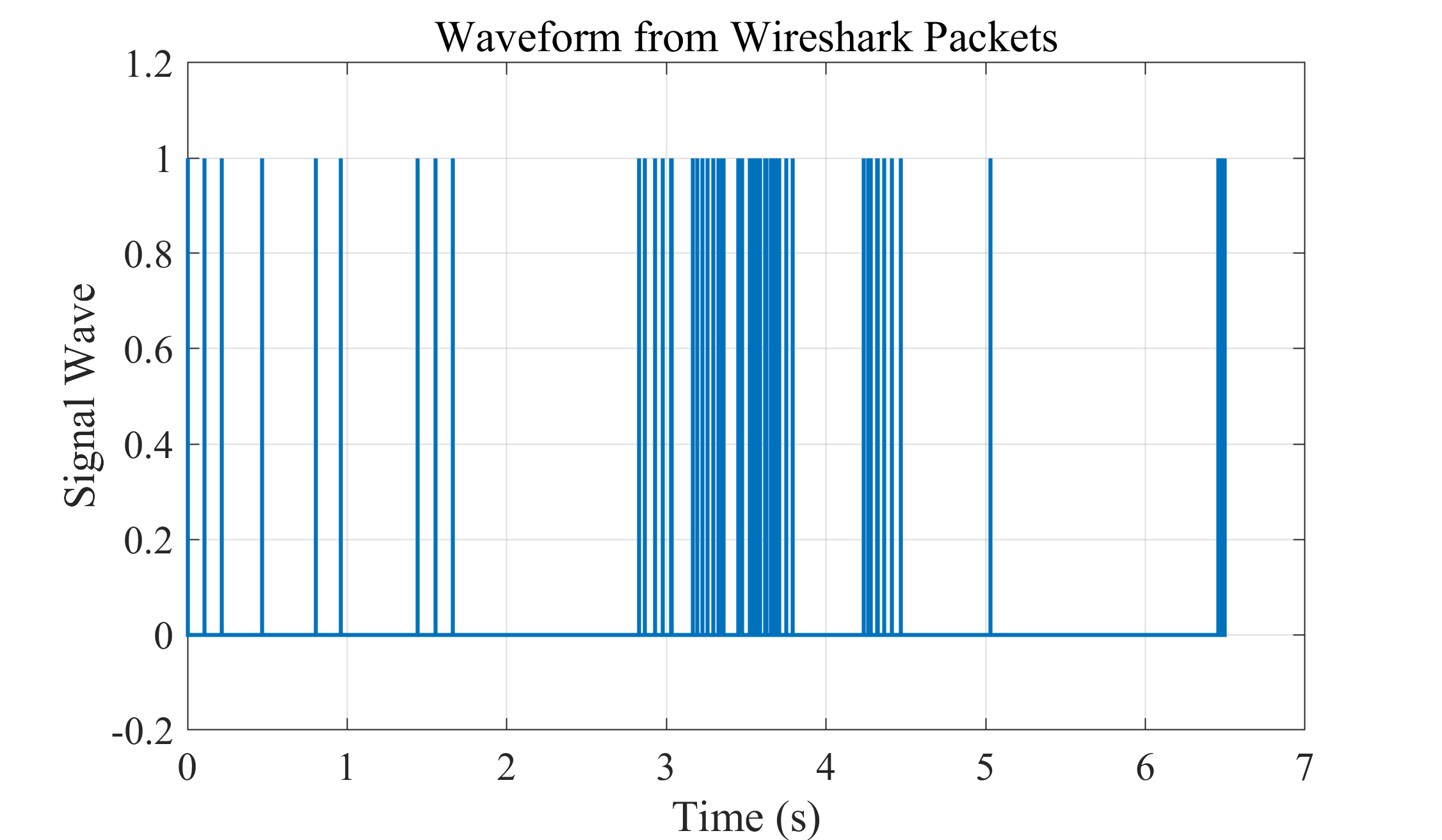
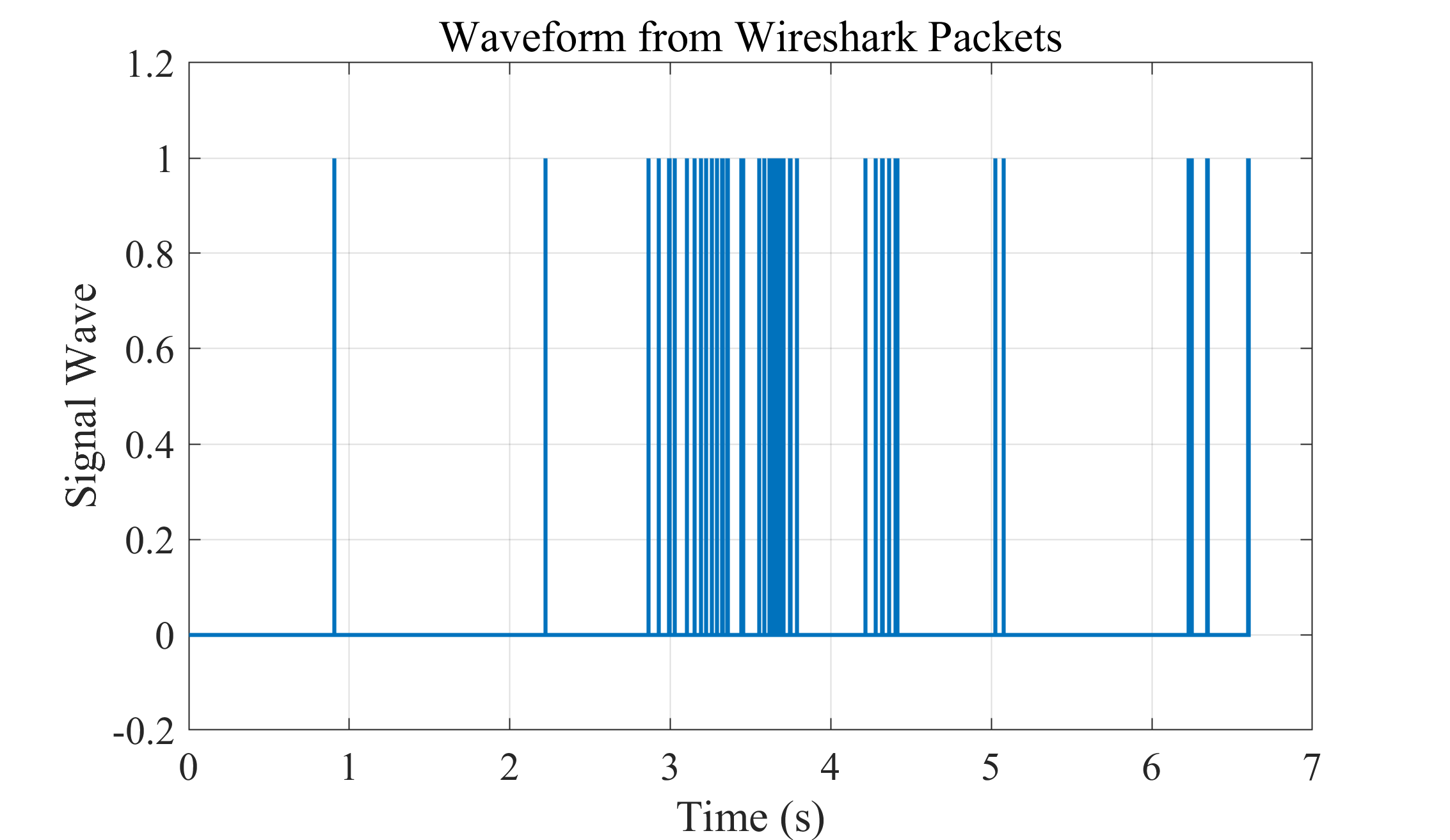
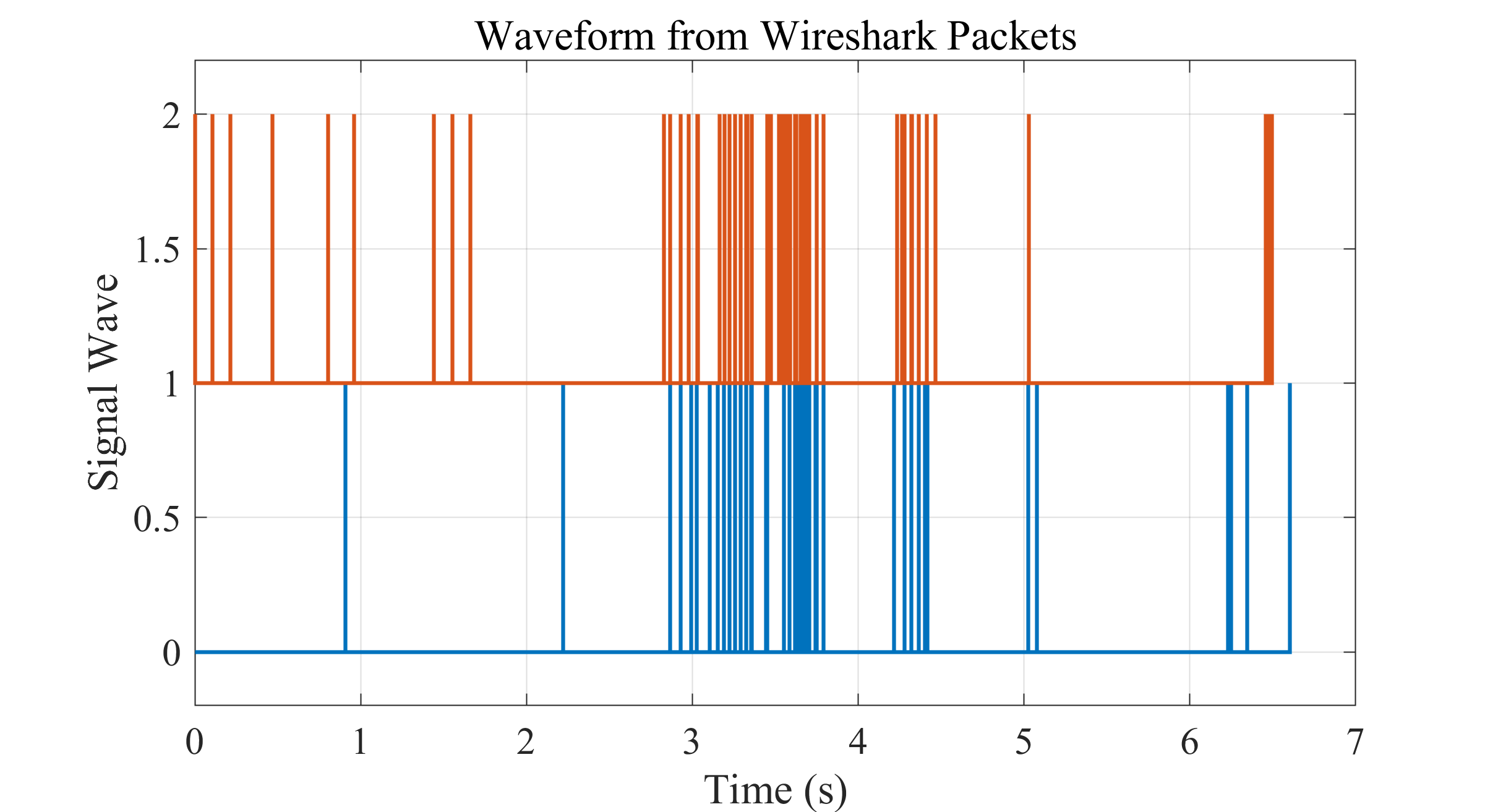
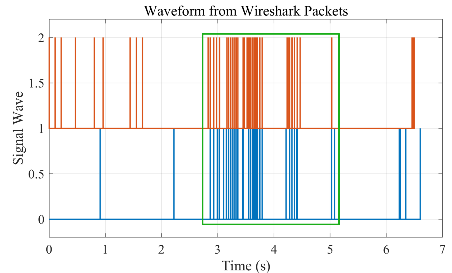
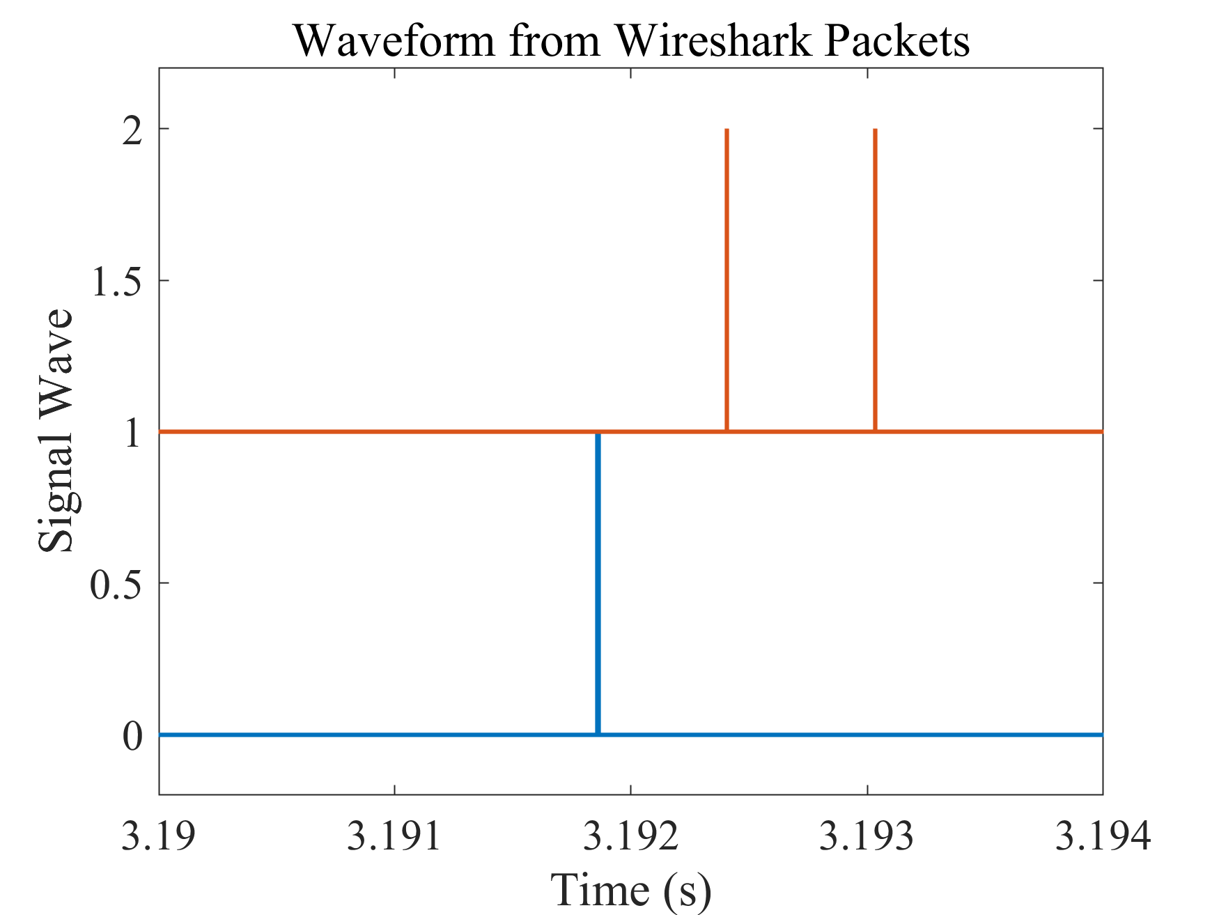
set(gca, 'FontSize', 15)save("D:\无线通信网络认知\通信学报\5G信号\Wireshark波形绘制\save_test.mat","t_plot","y_plot")source=192.168.1.103的波形和direction=192.168.1.103的波形,其中上面是我的电脑发出的信号波形,下面是我的电脑收到的信号波形(路由器发送):
三、波形多尺度观察
绿色框里电脑和路由器的波形表现出明显的相互性:
但是黄色框里电脑和路由器的波形显现得比较独立:
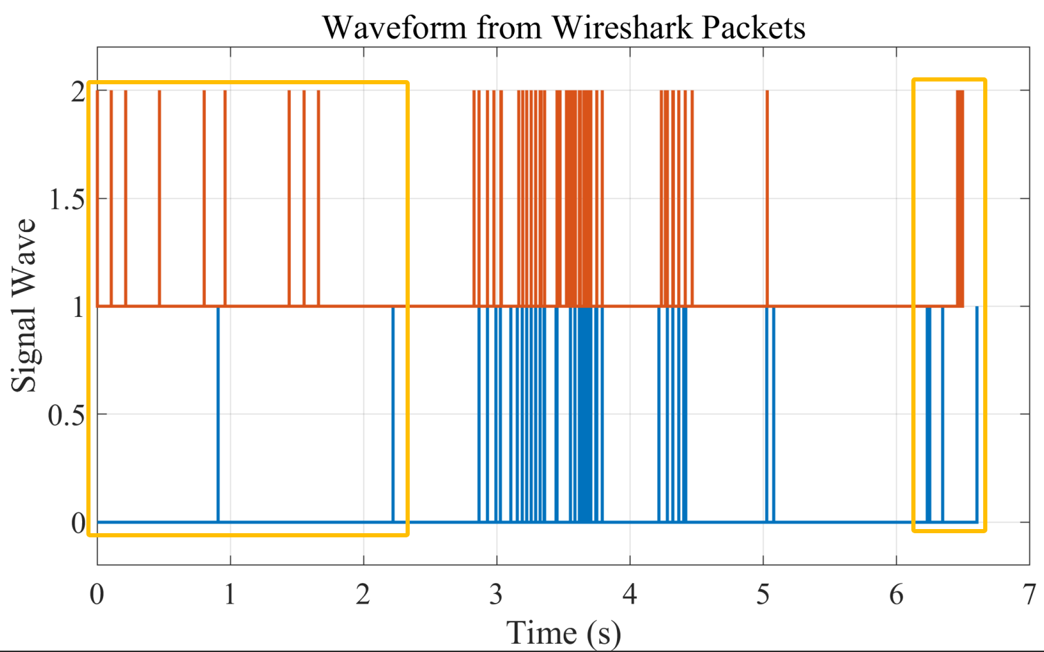
最前面我的电脑(红色)发了好多波形,路由器没响应;最后这个其实响应还比较明显,路由器(蓝色)发了很多数据,电脑收到后逐个响应。
放大波形看看:
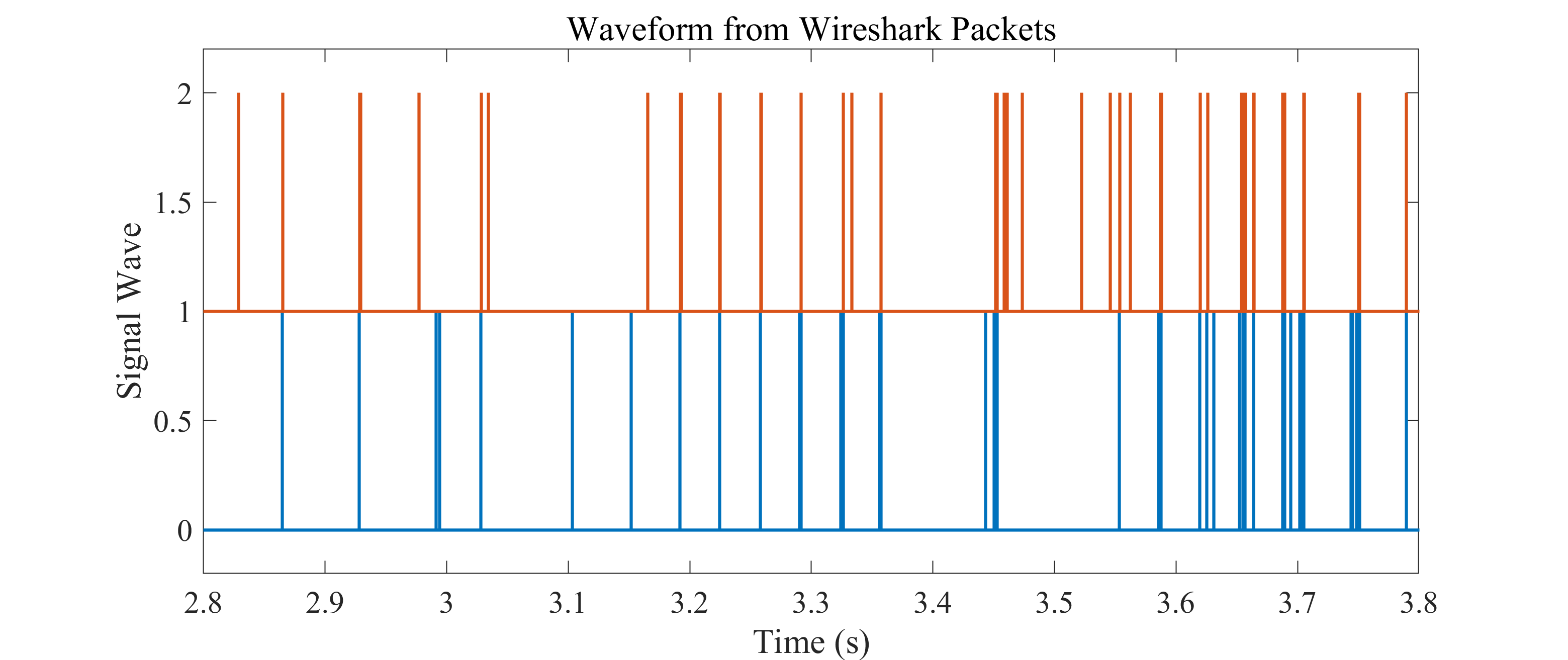
[3.1, 3.3]
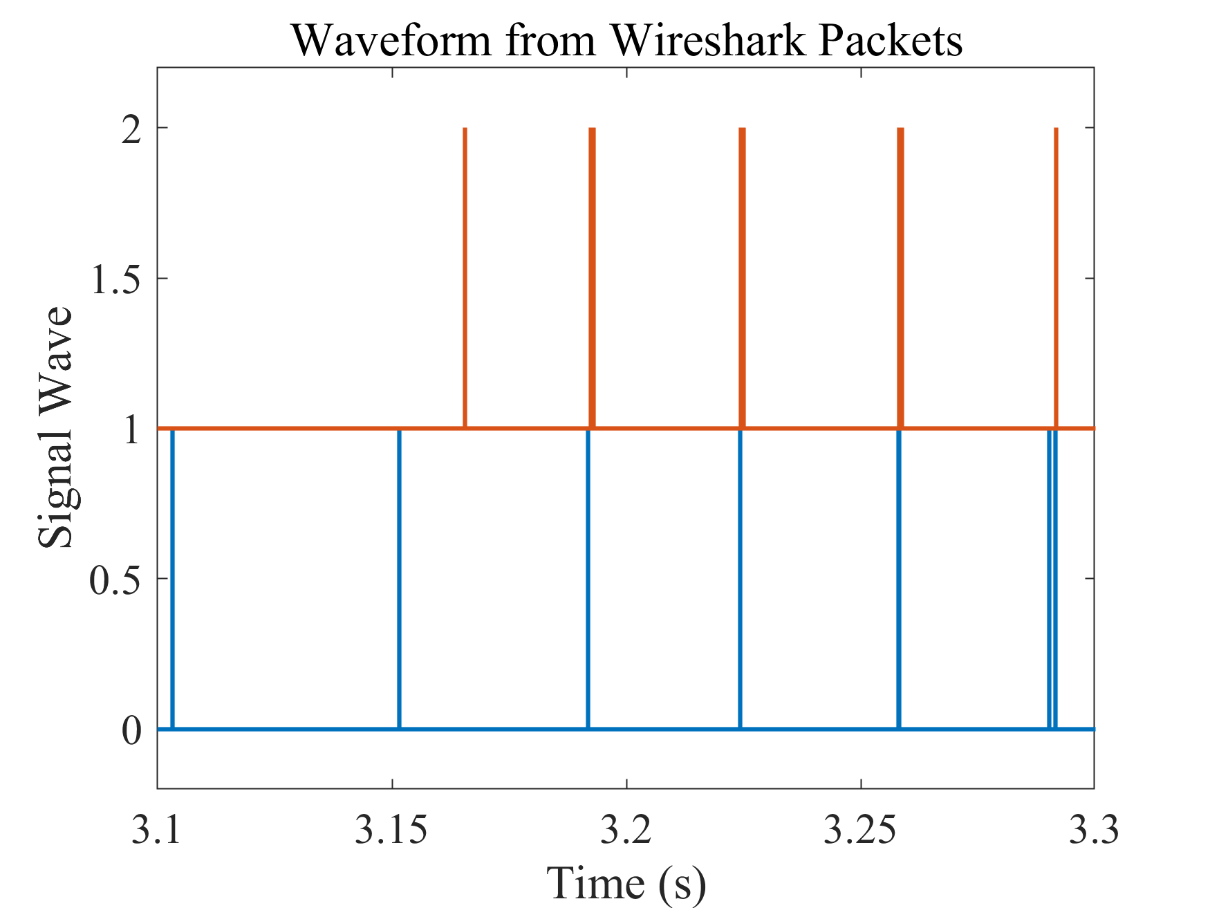
[3.19, 3.194]
xlim([3.19184,3.19187])
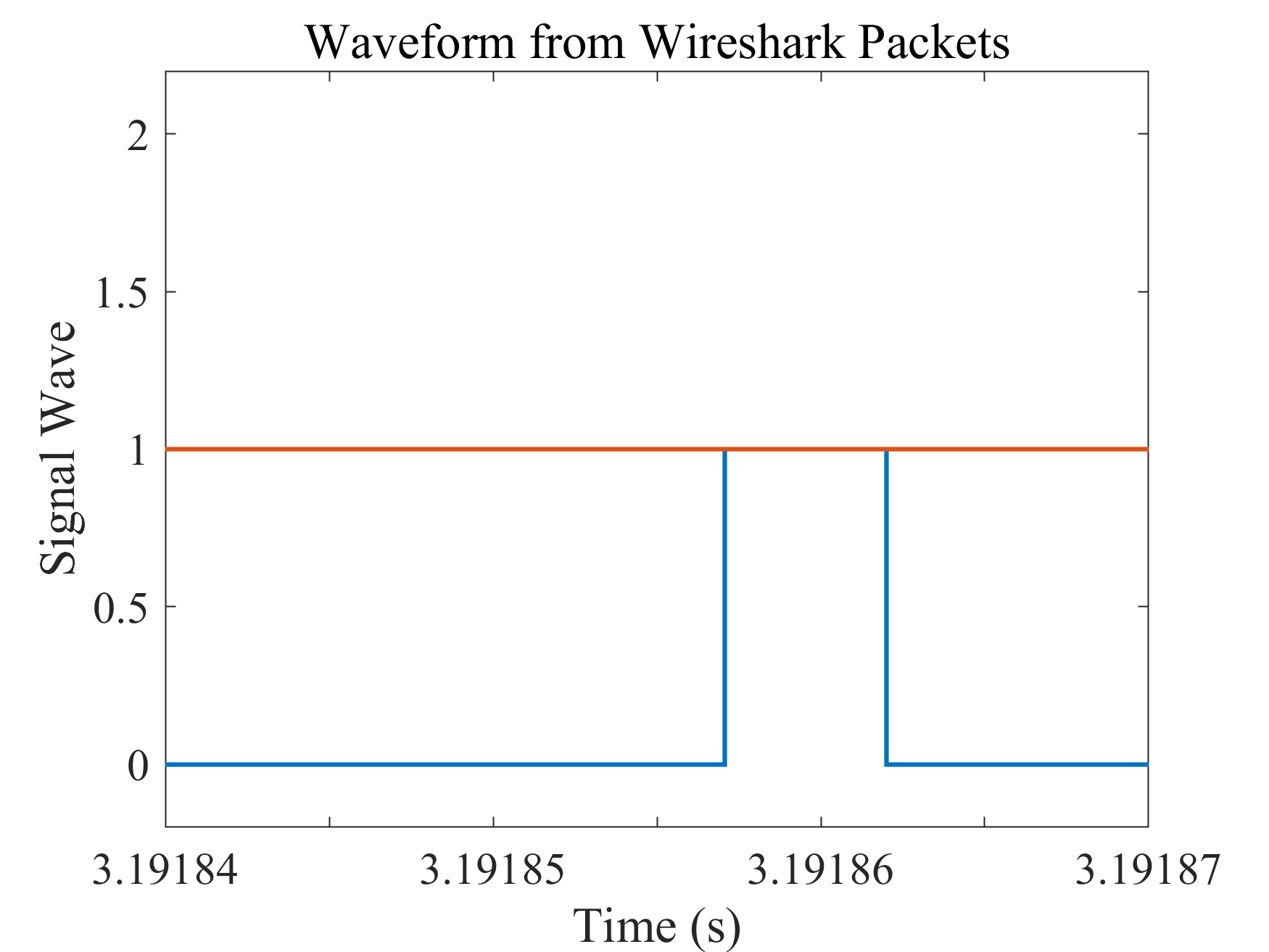
四、搭上载波
[3.19184,3.19187]这段信号时长3.19187-3.19184=0.00003s=0.03ms=30ns
2.4GHz下设置24GHz的采样率的话
0.00003s*24GHz=0.00003*24*10^9=720000采样点=72万个采样点
试试能不能仿真出来:
4.1 截取信号
首先把y_plot_1,t_plot_1在[3.19184,3.19187]进行截取:
%% 截取信号
% 定义时间区间
t_start = 3.19184;
t_end = 3.19187;% 找到在这个时间区间内的索引
indices = t_plot_1 >= (t_start-0.1) & t_plot_1 <= (t_end+0.1);% 截取数据
t_plot_1_segment = t_plot_1(indices);
y_plot_1_segment = y_plot_1(indices);% 绘制截取后的波形
figure;
stairs(t_plot_1_segment, y_plot_1_segment, 'LineWidth', 1.5);
xlim([t_start, t_end]);
ylim([-0.2, 2.2]);
xlabel('Time (s)');
ylabel('Signal Wave');
title('Segmented Waveform from Wireshark Packets');
set(gca, 'FontName', 'Times New Roman');
set(gca, 'FontSize', 15);
再绘制波形:
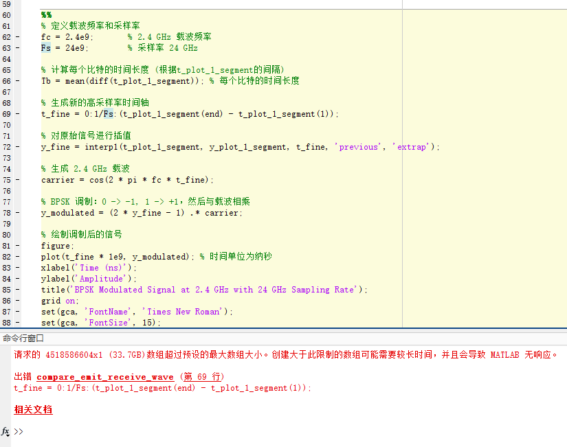
MATLAB直接仿真2.4GHz的载波有些太困难了。
降低采样率:
% 定义载波频率和采样率
fc = 2.4e9;       % 2.4 GHz 载波频率
Fs = 5e9;        % 采样率 24 GHz
4.2 时间轴递增
K>> fprintf('%.8f\n', t_plot_1_segment(1));
3.10319956
K>> fprintf('%.8f\n', t_plot_1_segment(2));
3.10319956
K>> fprintf('%.8f\n', t_plot_1_segment(3));
3.10320100
K>> fprintf('%.8f\n', t_plot_1_segment(4));
3.10320100
把t轴上一样的数值第一次出现时-0.00001:
% 初始偏移量
offset = 0.00001;% 初始化一个新数组,用于存储调整后的值
t_plot_1_segment_adjusted = t_plot_1_segment;% 遍历 `t_plot_1_segment` 数组
for i = 2:length(t_plot_1_segment)% 如果当前值与前一个值相同,调整当前值if t_plot_1_segment_adjusted(i) == t_plot_1_segment_adjusted(i-1)t_plot_1_segment_adjusted(i-1) = t_plot_1_segment_adjusted(i-1) - offset;end
end
4.3 插值
插值思路:
对y_plot_1_segment和t_plot_1_segment_adjusted进行插值。
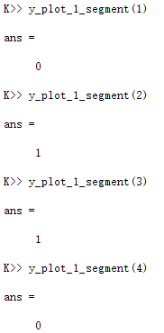
首先检查y_plot_1_segment中的两个挨在一起的1,中间补充1,补充1的数量根据两个挨在一起的1对应的t_plot_1_segment_adjusted中的数值差,和采样率Fs计算;
然后,检查y_plot_1_segment中的两个挨在一起的0,中间补充0,补充0的数量根据两个挨在一起的0对应的t_plot_1_segment_adjusted中的数值差,和采样率Fs计算;
最后,检查y_plot_1_segment中的两个挨在一起的0和1,0和1之间补充0,补充0的数量根据两个挨在一起的0对应的t_plot_1_segment_adjusted中的数值差,和采样率Fs计算。
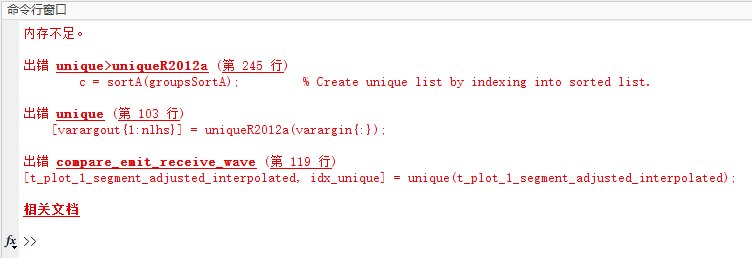
内存还是不够,降低中心频率和采样率:
% 定义载波频率和采样率
fc = 1.2e9;       % 2.4 GHz 载波频率
Fs = 39;        % 采样率 24 GHz
4.4 电磁波
本来还想在调制载波之后优化为电磁波图:
(27 封私信) 用什么软件能画出这样的图? - 知乎
x = (0:2:300)/50;
y = -sin(x*pi); z = cos(x*pi);
[m,M] = cellfun(@(t)deal(min(t),max(t)),{x,y,z});
[yc,zc,xc] = cylinder(1,500); xc = xc*M(1);
figure('render','painter','color','w'), view(44,14), axis image ij off, hold on
line(x,y,z,'linewidth',2,'color','r')
line(xc',yc',zc','color',[1 0.7 0.7])
h = surface(xc,yc,zc,'facecolor','none','edgecolor','r','edgealpha',0.02);
quiver3(x,0*x,0*z,0*x,y,z,0,'k','linewidth',1,'maxhead',0.06);
quiver3([m(1) 0 0],[0 m(2) 0],[0 0 m(3)],...[1.2*(M(1)-m(1)) 0 0],[0 1.3*(M(2)-m(2)) 0],[0 0 1.3*(M(3)-m(3))],0,...'linewidth',2,'color','k','maxhead',0.08)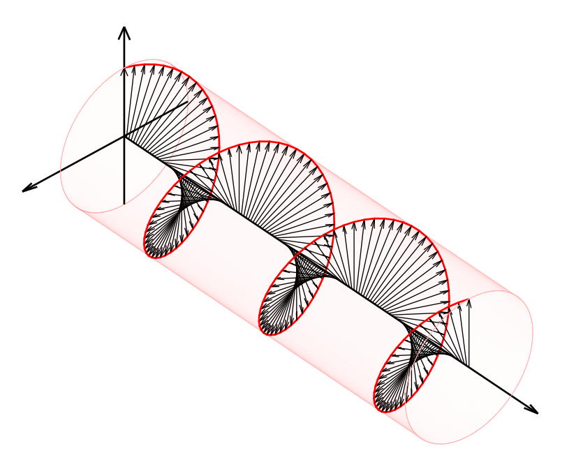
现在连载波也仿真不出。
的一种方案)


——VGA显示彩条和图片)

![week2-[一维数组]出现次数](http://pic.xiahunao.cn/week2-[一维数组]出现次数)


)