大熊猫卸妆后
数据科学 (Data Science)
Pandas is used mainly for reading, cleaning, and extracting insights from data. We will see an advanced use of Pandas which are very important to a Data Scientist. These operations are used to analyze data and manipulate it if required. These are used in the steps performed before building any machine learning model.
熊猫主要用于读取,清洁和从数据中提取见解。 我们将看到对数据科学家非常重要的熊猫的高级用法。 这些操作用于分析数据并根据需要进行操作。 这些用于构建任何机器学习模型之前执行的步骤。
- Summarising Data 汇总数据
- Concatenation 级联
- Merge and Join 合并与加入
- Grouping 分组
- Pivot Table 数据透视表
- Reshaping multi-index DataFrame 重塑多索引DataFrame
We will be using the very famous Titanic dataset to explore the functionalities of Pandas. Let’s just quickly import NumPy, Pandas, and load Titanic Dataset from Seaborn.
我们将使用非常著名的泰坦尼克号数据集来探索熊猫的功能。 让我们快速导入NumPy,Pandas,并从Seaborn加载Titanic Dataset。
import numpy as np
import pandas as pd
import seaborn as snsdf = sns.load_dataset('titanic')
df.head()
汇总数据 (Summarizing data)
The very first thing any data scientist would like to know is the statistics of the entire data. With the help of the Pandas .describe() method, we can see the summary stats of each feature. Notice, the stats are given only for numerical columns which is an obvious behavior we can also ask describe function to include categorical columns with the parameter ‘include’ and value equal to ‘all’ ( include=‘all’).
任何数据科学家都想知道的第一件事就是整个数据的统计信息。 借助Pandas .describe()方法 ,我们可以看到每个功能的摘要状态。 注意,仅针对数字列提供统计信息,这是显而易见的行为,我们也可以要求describe函数包括参数为'include'并且值等于'all'(include ='all')的分类列。
df.describe()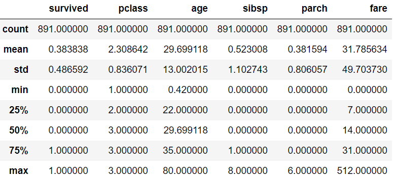
Another method is .info(). It gives metadata of a dataset. We can see the size of the dataset, dtype, and count of null values in each column.
另一个方法是.info() 。 它给出了数据集的元数据。 我们可以在每个列中看到数据集的大小,dtype和空值的计数。
df.info()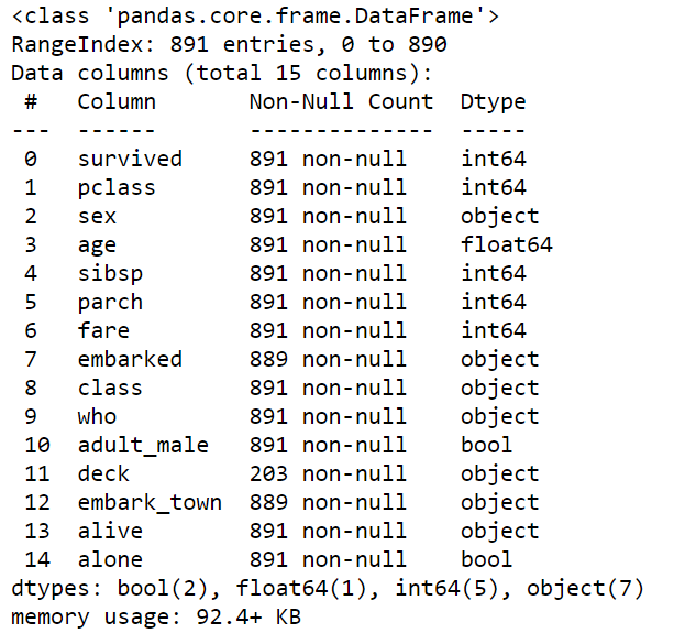
级联 (Concatenation)
Concatenation of two DataFrames is very straightforward, thanks to the Pandas method concat(). Let us take a small section of our Titanic data with the help of vector indexing. Vector indexing is a way to specify the row and column name/integer we would like to index in any order as a list.
借助于Pandas 方法concat() ,两个DataFrame的串联非常简单。 让我们在矢量索引的帮助下,提取一小部分Titanic数据。 扇区索引是一种指定行和列名称/整数的方法,我们希望以列表的任何顺序对其进行索引。
smallData = df.loc[[1,7,21,10], ['sex','age','fare','who','class']]
smallData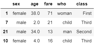
Also, I have created a dataset with matching columns to explain concatenation.
另外,我还创建了带有匹配列的数据集来说明串联。
newData = pd.DataFrame({’sex’:[’female’,’male’,’male’],’age’: [25,49,35], ’fare’:[89.22,70.653,30.666],’who’:[’child’, 'women’, 'man’],'class’:[’First’,’First’,’First’]})
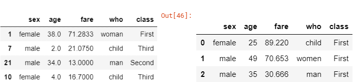
By default, the concatenation happens row-wise. Let’s see how the new dataset looks when we concat the two DataFrames.
默认情况下,串联是逐行进行的 。 让我们看看当连接两个DataFrame时新数据集的外观。
pd.concat([smallData, newData])
What if we want to concatenate ignoring the index? just set the ingore_index parameter to True.
如果我们想串联忽略索引怎么办? 只需将ingore_index参数设置为True。
pd.concat([ newData,smallData], ignore_index=True)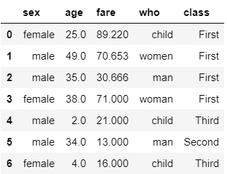
If we wish to concatenate along with the columns we just have to change the axis parameter to 1.
如果我们希望与列连接在一起,我们只需要将axis参数更改为1。
pd.concat([ newData,smallData], axis=1)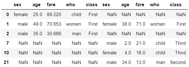
Notice the changes? As soon we concatenated column-wise Pandas arranged the data in an order of row indices. In smallData, row 0 and 2 are missing but present in newData hence insert them in sequential order. But we have row 1 in both the data and Pandas retained the data of the 1st dataset because that was the 1st dataset we passed as a parameter to concat. Also, the missing data is represented as NaN.
注意到变化了吗? 一旦我们串联列式熊猫,便以行索引的顺序排列了数据。 在smallData中,缺少第0行和第2行,但存在于newData中,因此按顺序插入它们。 但是我们在数据中都有第1行,Pandas保留了第一个数据集的数据,因为那是我们作为参数传递给concat的第一个数据集。 同样,缺失的数据表示为NaN。
We can also perform concatenation in SQL join fashion. Let’s create a new DataFrame ‘newData’ having a few columns the same as smallData but not all.
我们还可以以SQL连接的方式执行串联。 让我们创建一个新的DataFrame'newData',其中有几列与smallData相同,但并非全部。
newData = pd.DataFrame({'fare':[89.22,70.653,30.666,100],
                        'who':['child', 'women', 'man', 'women'],
                        'class':['First','First','First','Second'],
                       'adult_male': [True, False, True, False]})
newData
If you are familiar with SQL join operation we can notice that .concat() performs outer join by default. Missing values for unmatched columns are filled with NaN.
如果您熟悉SQL连接操作,我们会注意到.concat()默认执行外部连接 。 未匹配列的缺失值用NaN填充。
pd.concat([smallData, newData])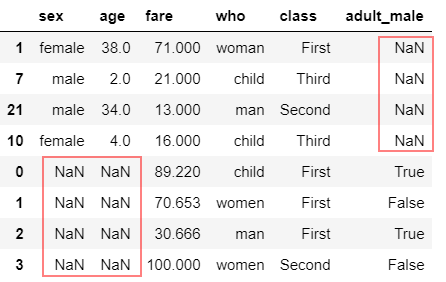
We can control the type of join operation with ‘join’ parameter. Let’s perform an inner join that takes only common columns from two.
我们可以使用'join'参数控制联接操作的类型。 让我们执行一个内部联接,该联接只接受两个公共列。
pd.concat([smallData, newData], join='inner')
Merge and Join
合并与加入
Pandas provide us an exclusive and more efficient method .merge() to perform in-memory join operations. Merge method is a subset of relational algebra that comes under SQL.
熊猫为我们提供了一种排他的,更有效的方法.merge()来执行内存中的联接操作。 合并方法是SQL下的关系代数的子集。
I will be moving away from our Titanic dataset only for this section to ease the understanding of join operation with less complex data.
在本节中,我将不再使用Titanic数据集,以简化对不太复杂数据的联接操作的理解。
There are different types of join operations:
有不同类型的联接操作:
- One-to-one 一对一
- Many-to-one 多对一
- Many-to-many 多对多
The classic data used to explain joins in SQL in the employee dataset. Lets create DataFrames.
用于解释员工数据集中SQL中联接的经典数据。 让我们创建DataFrames。
df1=pd.DataFrame({'employee_name'['Tasha','Linda','Olliver','Jack'],'department':['Engineering', 'Accounting', 'HR', 'HR']})df2 = pd.DataFrame({'employee_name':['Linda', 'Tasha', 'Jack', 'Olliver'],'salary':[35000, 20500, 90000, 68000]})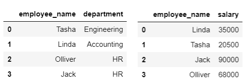
One-to-one
一对一
One-to-one merge is very similar to column-wise concatenation. To combine ‘df1’ and ‘df2’ we use .merge() method. Merge is capable of recognizing common columns in the datasets and uses it as a key, in our case column ‘employee_name’. Also, the names are not in order. Let’s see how the merge does the work for us by ignoring the indices.
一对一合并与按列合并非常相似。 要组合'df1'和'df2',我们使用.merge()方法。 合并能够识别数据集中的公共列 ,并将其用作键 (在我们的示例中为“ employee_name”列)。 另外,名称不正确。 让我们看看合并如何通过忽略索引为我们工作。
df3 = pd.merge(df1,df2)
df3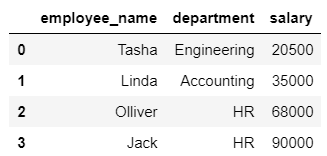
Many-to-one
多对一
Many-to-one is a type of join in which one of the two key columns have duplicate values. Suppose we have supervisors for each department and there are many employees in each department hence, Many employees to one supervisor.
多对一是一种连接类型,其中两个键列之一具有重复值 。 假设我们每个部门都有主管,每个部门有很多员工,因此, 一个主管有很多员工。
df4 = pd.DataFrame({'department':['Engineering', 'Accounting', 'HR'],'supervisor': ['Jonas', 'Martha', 'Martin']})print('--------df4---------\n',df4)print('-------merged--------')pd.merge(df3, df4)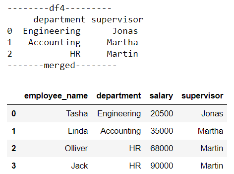
Many-to-many
多对多
This is the case where the key column in both the dataset has duplicate values. Suppose many skills are mapped to each department then the resulting DataFrame will have duplicate entries.
这是两个数据集中的键列都有重复值的情况 。 假设每个部门都有许多技能,那么生成的DataFrame将具有重复的条目。
df5=pd.DataFrame({'department'['Engineering','Engineering','Accounting','Accounting', 'HR', 'HR'],'skills': ['Coding', 'Soft skills', 'Math', 'Excel', 'Organizing', 'Decision making']})print('--------df5---------\n',df5)print('\n-------merged--------')pd.merge(df3, df5)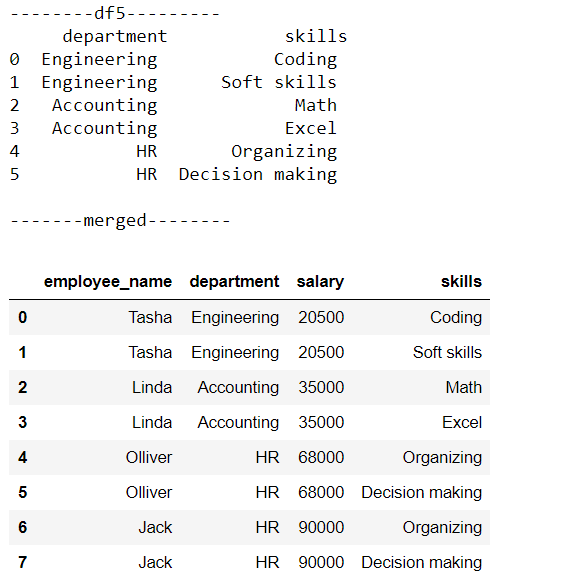
合并不常见的列名称和值 (Merge on uncommon column names and values)
Uncommon column names
罕见的列名
Many times merging is not that simple since the data we receive will not be so clean. We saw how the merge does all the work provided we have one common column. What if we have no common columns at all? or there is more than one common column. Pandas provide us the flexibility to explicitly specify the columns to act as the key in both DataFrames.
很多时候合并不是那么简单,因为我们收到的数据不会那么干净。 我们看到合并是如何完成所有工作的,只要我们有一个共同的专栏即可。 如果我们根本没有公共列怎么办? 或有多个共同的栏目 。 熊猫为我们提供了灵活地显式指定列以充当两个DataFrame中的键的灵活性。
Suppose we change our ‘employee_name’ column to ‘name’ in ‘df2’. Let’s see how datasets look and how to tell merge explicitly the key columns.
假设我们在“ df2”中将“ employee_name”列更改为“ name”。 让我们看看数据集的外观以及如何明确地合并关键列。
df2 = pd.DataFrame({'name':['Linda', 'Tasha', 'Jack', 'Olliver'],
                    'salary':[35000, 20500, 90000, 68000]})print('--------df1---------\n',df1)print('--------df2---------\n',df2)print('\n-------merged--------')pd.merge(df1, df2, left_on='employee_name', right_on='name')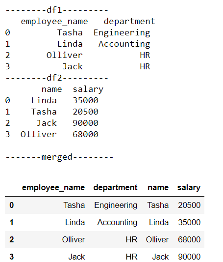
Parameter ‘left_on’ to specify the key of the first column and ‘right_on’ for the key of the second. Remember, the value of ‘left_on’ should match with the columns of the first DataFrame you passed and ‘right_on’ with second. Notice, we get redundant column ‘name’, we can drop it if not needed.
参数'left_on'指定第一列的键,'right_on'指定第二列的键。 请记住,“ left_on”的值应与您传递的第一个DataFrame的列匹配,第二个则与“ right_on”的列匹配。 注意,我们得到了多余的列“名称”,如果不需要的话可以将其删除。
Uncommon values
罕见的价值观
Previously we saw that all the employee names present in one dataset were also present in other. What if the names are missing.
以前,我们看到一个数据集中存在的所有雇员姓名也存在于另一个数据集中。 如果缺少名称怎么办。
df1=pd.DataFrame({'employee_name'['Tasha','Linda','Olliver','Jack'],  'department':['Engineering', 'Accounting', 'HR', 'HR']})
df2 = pd.DataFrame({'employee_name':['Linda', 'Mary'],'salary':[35000, 20500]})print('--------df1---------\n',df1)print('--------df2---------\n',df2)print('\n-------merged--------\n')pd.merge(df1, df2)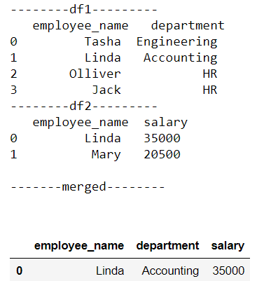
By default merge applies inner join, meaning join in performed only on common values which is always not preferred way since there will be data loss. The method of joining can be controlled by using the parameter ‘how’. We can perform left join or right join to overcome data loss. The missing values will be represented as NaN by Pandas.
默认情况下,合并将应用内部联接 ,这意味着联接仅在通用值上执行,由于存在数据丢失,因此始终不建议采用这种方式。 可以通过使用参数“如何”来控制加入方法。 我们可以执行左联接或右联接以克服数据丢失。 缺失值将由Pandas表示为NaN。
print('-------left join--------\n',pd.merge(df1, df2, how='left'))
print('\n-------right join--------\n',pd.merge(df1,df2,how='right'))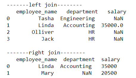
通过...分组 (GroupBy)
GroupBy is a very flexible abstraction, we can think of it as a collection of DataFrame. It allows us to do many different powerful operations. In simple words, it groups the entire data set by the values of the column we specify and allows us to perform operations to extract insights.
GroupBy是一个非常灵活的抽象,我们可以将其视为DataFrame的集合。 它允许我们执行许多不同的强大操作。 简而言之,它通过我们指定的列的值对整个数据集进行分组,并允许我们执行操作以提取见解。
Let’s come back to our Titanic dataset
让我们回到泰坦尼克号数据集
Suppose we would like to see how many male and female passengers survived.
假设我们想看看有多少男女乘客幸存下来。
print(df.groupby('sex'))
df.groupby('sex').sum()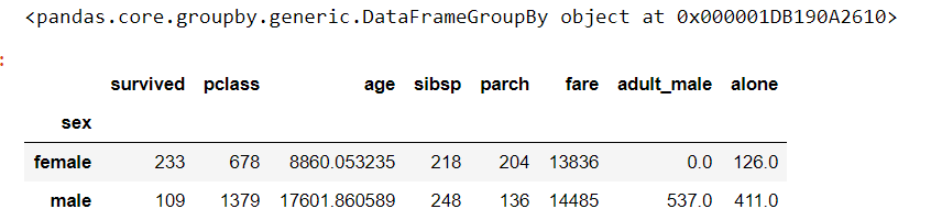
Notice, printing only the groupby without performing any operation gives GroupBy object. Since there are only two unique values in the column ‘sex’ we can see a summation of every other column grouped by male and female. More insightful would be to get the percentage. We will capture only the ‘survived’ column of groupby result above upon summation and calculate percentages.
注意,仅打印groupby而不执行任何操作将给出GroupBy对象。 由于“性别”列中只有两个唯一值,因此我们可以看到按性别分组的所有其他列的总和。 更有见地的将是获得百分比。 求和后,我们将仅捕获以上groupby结果的“幸存”列,并计算百分比。
data = df.groupby('sex')['survived'].sum()print('% of male survivers',(data['male']/(data['male']+data['female']))*100)print('% of male female',(data['female']/(data['male']+data['female']))*100)Output% of male survivers 31.87134502923976
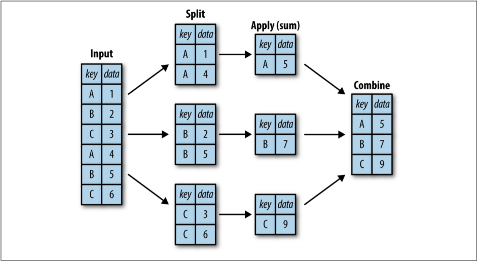
% of male female 68.12865497076024Under the hood, the GroupBy function performs three operations: split-apply-combine.
在幕后,GroupBy函数执行三个操作: split-apply-combine。
- Split - breaking the DataFrame in order to group it into the specified key. 拆分-拆分DataFrame以便将其分组为指定的键。
- Apply - it involves computing the function we wish like aggregation or transformation or filter. 应用-它涉及计算我们希望的功能,例如聚合,转换或过滤。
- Combine - merging the output into a single DataFrame. 合并-将输出合并到单个DataFrame中。
Perhaps, more powerful operations that can be performed on groupby are:
也许可以对groupby执行的更强大的操作是:
- Aggregate 骨料
- Filter 过滤
- Transform 转变
- Apply 应用
Let’s see each one with an example.
让我们来看一个例子。
Aggregate
骨料
The aggregate function allows us to perform more than one aggregation at a time. We need to pass the list of required aggregates as a parameter to .aggregate() function.
聚合功能使我们可以一次执行多个聚合 。 我们需要将所需聚合的列表作为参数传递给.aggregate()函数。
df.groupby('sex')['survived'].aggregate(['sum', np.mean,'median'])
Filter
过滤
The filter function allows us to drop data based on group property. Suppose we want to see data where the standard deviation of ‘fare’ is greater than the threshold value say 50 when grouped by ‘survived’.
过滤器功能使我们可以基于组属性删除数据 。 假设我们想查看“票价”的标准偏差大于按“生存”分组的阈值(例如50)的数据。
df.groupby('survived').filter(lambda x: x['fare'].std() > 50)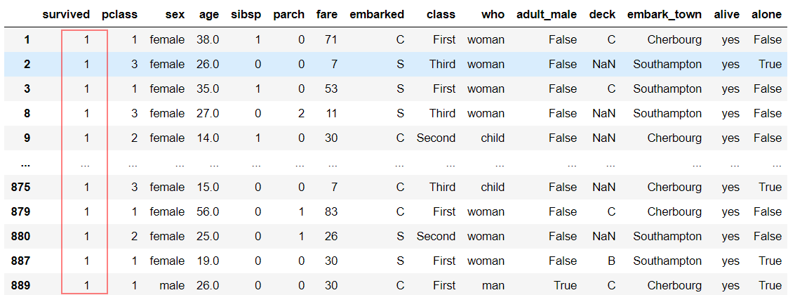
Since the standard deviation of ‘fare’ is greater than 50 only for values of ‘survived’ equal to 1, we can see data only where ‘survived’ is 1.
由于仅当“ survived”等于1时,“ fare”的标准差才大于50,因此我们只能在“ survived”为1的情况下才能看到数据。
Transform
转变
Transform returns the transformed version of the entire data. The best example to explain is to center the dataset. Centering the data is nothing but subtracting each value of the column with the mean value of its respective column.
转换返回整个数据的转换版本 。 最好的解释示例是将数据集居中。 使数据居中无非是用该列的各个值的平均值减去该列的每个值。
df.groupby('survived').transform(lambda x: x - x.mean())
Apply
应用
Apply is very flexible unlike filter and transform, the only criteria are it takes a DataFrame and returns Pandas object or scalar. We have the flexibility to do anything we wish in the function.
Apply与过滤器和变换不同,它非常灵活,唯一的条件是它需要一个DataFrame并返回Pandas对象或标量。 我们可以灵活地执行该函数中希望执行的任何操作。
def func(x):
    x['fare'] = x['fare'] / x['fare'].sum()
    return xdf.groupby('survived').apply(func)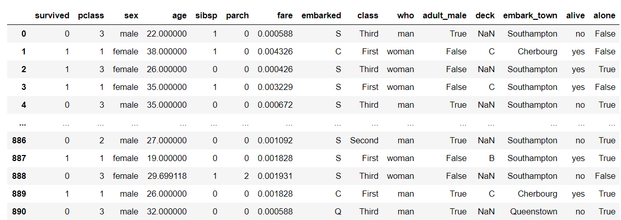
数据透视表 (Pivot tables)
Previously in GroupBy, we saw how ‘sex’ affected survival, the survival rate of females is much larger than males. Suppose we would also like to see how ‘pclass’ affected the survival but both ‘sex’ and ‘pclass’ side by side. Using GroupBy we would do something like this.
之前在GroupBy中,我们看到了“性别”如何影响生存,女性的生存率远高于男性。 假设我们还想了解“ pclass”如何影响生存,但“ sex”和“ pclass”并存。 使用GroupBy,我们将执行以下操作。
df.groupby(['sex', 'pclass']['survived'].aggregate('mean').unstack()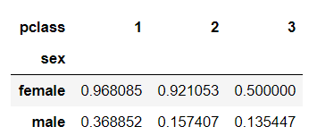
This is more insightful, we can easily make out passengers in the third class section of the Titanic are less likely to be survived.
这是更有洞察力的,我们可以很容易地看出,泰坦尼克号三等舱的乘客幸存下来的可能性较小。
This type of operation is very common in the analysis. Hence, Pandas provides the function .pivot_table() which performs the same with more flexibility and less complexity.
这种类型的操作在分析中非常常见。 因此,Pandas提供了.pivot_table()函数,该函数以更大的灵活性和更低的复杂度执行相同的功能。
df.pivot_table('survived', index='sex', columns='pclass')The result of the pivot table function is a DataFrame, unlike groupby which returned a groupby object. We can perform all the DataFrame operations normally on it.
数据透视表功能的结果是一个DataFrame,与groupby不同,后者返回了groupby对象。 我们可以正常执行所有DataFrame操作。
We can also add a third dimension to our result. Suppose we want to see how ‘age’ has also affected the survival rate along with ‘sex’ and ‘pclass’. Let’s divide our ‘age’ into groups within it: 0–18 child/teenager, 18–40 adult, and 41–80 old.
我们还可以在结果中添加第三维 。 假设我们想了解“年龄”如何同时影响“性别”和“ pclass”的生存率。 让我们将“年龄”分为几类:0-18岁的儿童/青少年,18-40岁的成人和41-80岁的孩子。
age = pd.cut(df['age'], [0, 18, 40, 80])
pivotTable = df.pivot_table('survived', ['sex', age], 'class')
pivotTable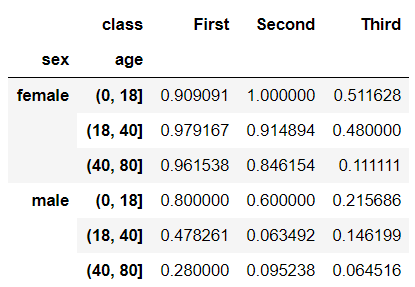
Interestingly female children and teenagers in the second class have a 100% survival rate. This is the kind of power the pivot table of Pandas has.
有趣的是,二等班的女孩和青少年的存活率是100%。 这就是Pandas数据透视表具有的功能。
重塑多索引DataFrame (Reshaping Multi-index DataFrame)
To see a multi-index DataFrame from a different view we reshape it. Stack and Unstack are the two methods to accomplish this.
为了从不同的视图查看多索引DataFrame,我们对其进行了重塑。 Stack和Unstack是完成此操作的两种方法。
unstack( )
取消堆叠()
It is the process of converting the row index to the column index. The pivot table we created previously is multi-indexed row-wise. We can get the innermost row index(age groups) into the innermost column index.
这是将行索引转换为列索引的过程。 我们之前创建的数据透视表是多索引的。 我们可以将最里面的行索引(年龄组)转换为最里面的列索引。
pivotTable = pivotTable.unstack()
pivotTable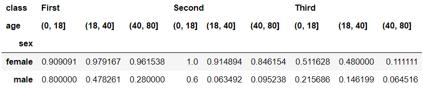
We can also convert the outermost row index(sex) into the innermost column index by using parameter ‘level’.
我们还可以通过使用参数“级别”将最外面的行索引(性别)转换为最里面的列索引。
pivotTable = pivotTable.unstack(level=0)
piviotTable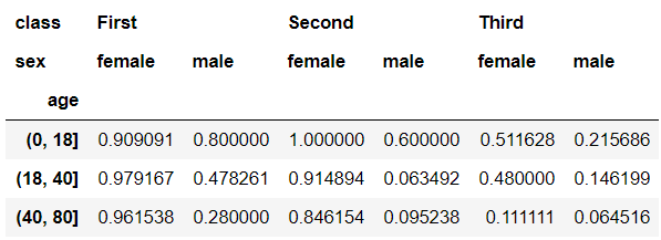
stack( )
堆栈()
Stacking is exactly inverse of unstacking. We can convert the column index of multi-index DataFrame into a row index. The innermost column index ‘sex’ is converted to the innermost row index. The result is slightly different from the original DataFrame because we unstacked with level 0 previously.
堆叠与堆叠完全相反。 我们可以将多索引DataFrame的列索引转换为行索引。 最里面的列索引“ sex”被转换为最里面的行索引。 结果与原始DataFrame略有不同,因为我们之前使用0级进行了堆叠。
pivotTable.stack()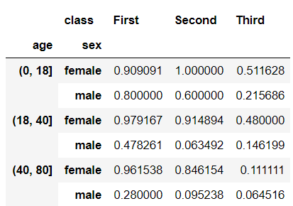
These functions and methods are very helpful to understand data, further used to manipulation, or to build a predictive model. We can also plot graphs to get visual insights.
这些功能和方法对于理解数据,进一步用于操纵或建立预测模型非常有帮助。 我们还可以绘制图形以获得视觉见解。
翻译自: https://medium.com/towards-artificial-intelligence/6-pandas-operations-you-should-not-miss-d531736c6574
大熊猫卸妆后
本文来自互联网用户投稿,该文观点仅代表作者本人,不代表本站立场。本站仅提供信息存储空间服务,不拥有所有权,不承担相关法律责任。 如若转载,请注明出处:http://www.pswp.cn/news/389431.shtml 繁体地址,请注明出处:http://hk.pswp.cn/news/389431.shtml 英文地址,请注明出处:http://en.pswp.cn/news/389431.shtml
如若内容造成侵权/违法违规/事实不符,请联系英文站点网进行投诉反馈email:809451989@qq.com,一经查实,立即删除!相关文章

数据eda_关于分类和有序数据的EDA

PyTorch官方教程中文版:PYTORCH之60MIN入门教程代码学习

Flexbox 最简单的表单


jdk重启后步行_向后介绍步行以一种新颖的方式来预测未来

PyTorch官方教程中文版:入门强化教程代码学习

css3-2 CSS3选择器和文本字体样式

mongodb仲裁者_真理的仲裁者

优化 回归_使用回归优化产品价格

Node.js——异步上传文件

用 JavaScript 的方式理解递归

PyTorch官方教程中文版:Pytorch之图像篇

大数据数据科学家常用面试题_进行数据科学工作面试

scrapy模拟模拟点击_模拟大流行

公司想申请网易企业电子邮箱,怎么样?

莫烦Matplotlib可视化第二章基本使用代码学习

vue.js python_使用Python和Vue.js自动化报告过程

plsql中导入csvs_在命令行中使用sql分析csvs

第十八篇 Linux环境下常用软件安装和使用指南
