某建筑和装饰板材的生产企业所用原材料主要是木质纤维和其他植物素纤维材料,
总体可分为 A,B,C 三种类型。该企业每年按 48 周安排生产,需要提前制定 24 周的原
材料订购和转运计划,即根据产能要求确定需要订购的原材料供应商(称为“供应商”)
和相应每周的原材料订购数量(称为“订货量”),确定第三方物流公司(称为“转运
商”)并委托其将供应商每周的原材料供货数量(称为“供货量”)转运到企业仓库。
该企业每周的产能为 2.82 万立方米,每立方米产品需消耗 A 类原材料 0.6 立方米,
或 B 类原材料 0.66 立方米,或 C 类原材料 0.72 立方米。由于原材料的特殊性,供应商
不能保证严格按订货量供货,实际供货量可能多于或少于订货量。为了保证正常生产的
需要,该企业要尽可能保持不少于满足两周生产需求的原材料库存量,为此该企业对供
应商实际提供的原材料总是全部收购。
在实际转运过程中,原材料会有一定的损耗(损耗量占供货量的百分比称为“损耗
率”),转运商实际运送到企业仓库的原材料数量称为“接收量”。每家转运商的运输
能力为 6000 立方米/周。通常情况下,一家供应商每周供应的原材料尽量由一家转运商
运输。
原材料的采购成本直接影响到企业的生产效益,实际中 A 类和 B 类原材料的采购单
价分别比 C 类原材料高 20%和 10%。三类原材料运输和储存的单位费用相同。
附件 1 给出了该企业近 5 年 402 家原材料供应商的订货量和供货量数据。附件 2 给
出了 8 家转运商的运输损耗率数据。请你们团队结合实际情况,对相关数据进行深入分
析,研究下列问题:
1.根据附件 1,对 402 家供应商的供货特征进行量化分析,建立反映保障企业生产
重要性的数学模型,在此基础上确定 50 家最重要的供应商,并在论文中列表给出结果。
2.参考问题 1,该企业应至少选择多少家供应商供应原材料才可能满足生产的需求?
针对这些供应商,为该企业制定未来 24 周每周最经济的原材料订购方案,并据此制定
损耗最少的转运方案。试对订购方案和转运方案的实施效果进行分析。
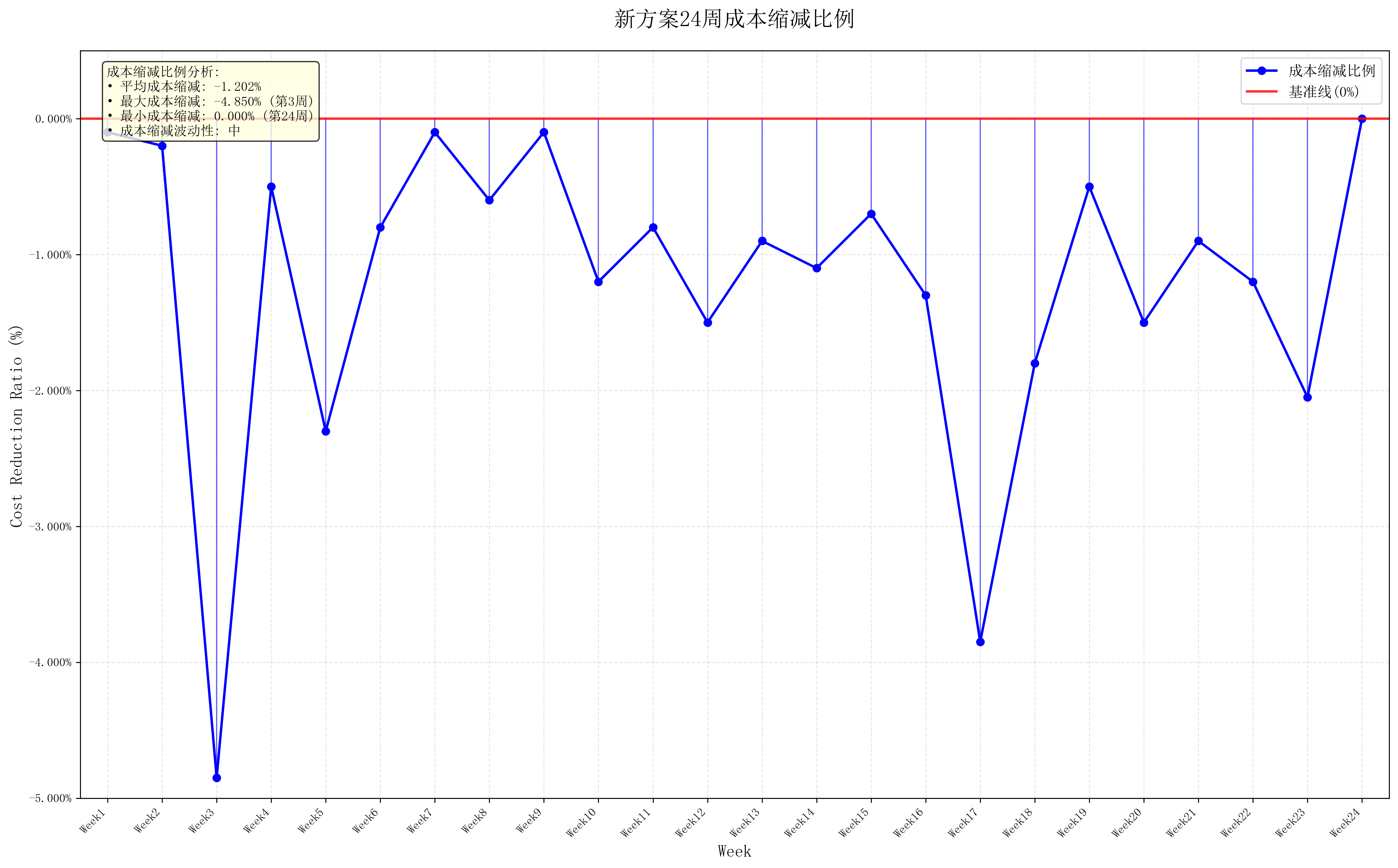
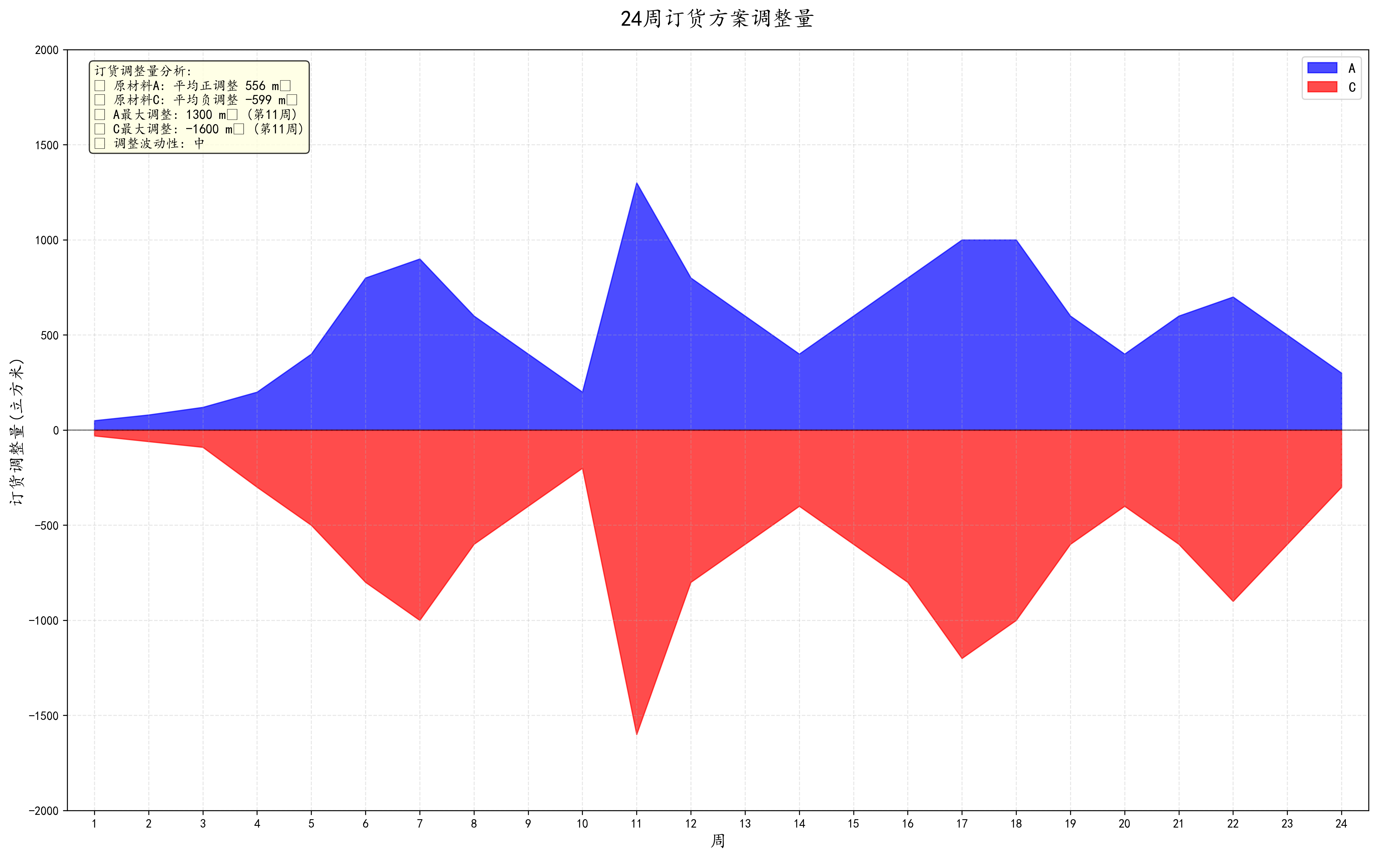
3.该企业为了压缩生产成本,现计划尽量多地采购 A 类和尽量少地采购 C 类原材
料,以减少转运及仓储的成本,同时希望转运商的转运损耗率尽量少。请制定新的订购
方案及转运方案,并分析方案的实施效果。
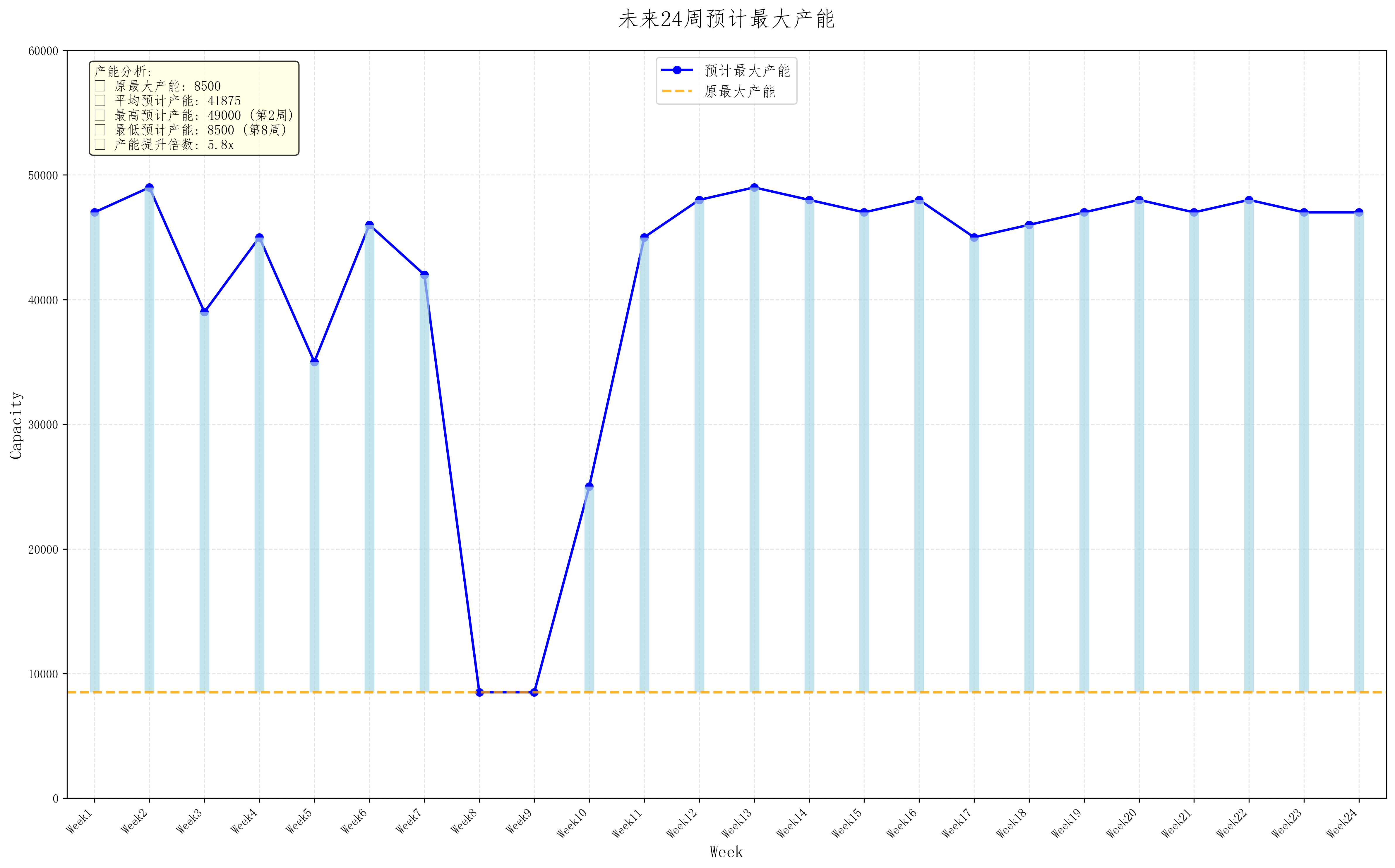
4.该企业通过技术改造已具备了提高产能的潜力。根据现有原材料的供应商和转运
商的实际情况,确定该企业每周的产能可以提高多少,并给出未来 24 周的订购和转运
方案。
1、数据预处理
import numpy as np
import pandas as pd
import mathdata = pd.DataFrame(pd.read_excel('附件1 近5年402家供应商的相关数据.xlsx', sheet_name=0))
data1 = pd.DataFrame(pd.read_excel('附件1 近5年402家供应商的相关数据.xlsx', sheet_name=1))data_a = data.loc[data['材料分类'] == 'A'].reset_index(drop=True)
data_b = data.loc[data['材料分类'] == 'B'].reset_index(drop=True)
data_c = data.loc[data['材料分类'] == 'C'].reset_index(drop=True)data1_a = data1.loc[data['材料分类'] == 'A'].reset_index(drop=True)
data1_b = data1.loc[data['材料分类'] == 'B'].reset_index(drop=True)
data1_c = data1.loc[data['材料分类'] == 'C'].reset_index(drop=True)data_a.to_excel('订货A.xlsx')
data_b.to_excel('订货B.xlsx')
data_c.to_excel('订货C.xlsx')data1_a.to_excel('供货A.xlsx')
data1_b.to_excel('供货B.xlsx')
data1_c.to_excel('供货C.xlsx')num_a = (data1_a == 0).astype(int).sum(axis=1)
num_b = (data1_b == 0).astype(int).sum(axis=1)
num_c = (data1_c == 0).astype(int).sum(axis=1)num_a = (240 - np.array(num_a)).tolist()
num_b = (240 - np.array(num_b)).tolist()
num_c = (240 - np.array(num_c)).tolist()total_a = data1_a.sum(axis=1).to_list()
total_b = data1_b.sum(axis=1).to_list()
total_c = data1_c.sum(axis=1).to_list()a = []
b = []
c = []
for i in range(len(total_a)):a.append(total_a[i] / num_a[i])
for i in range(len(total_b)):b.append(total_b[i] / num_b[i])
for i in range(len(total_c)):c.append(total_c[i] / num_c[i])data_a = pd.DataFrame(pd.read_excel('A.xlsx', sheet_name=1))
data_b = pd.DataFrame(pd.read_excel('B.xlsx', sheet_name=1))
data_c = pd.DataFrame(pd.read_excel('C.xlsx', sheet_name=1))a = np.array(data_a)
a = np.delete(a, [0, 1], axis=1)
b = np.array(data_b)
b = np.delete(b, [0, 1], axis=1)
c = np.array(data_c)
c = np.delete(c, [0, 1], axis=1)a1 = a.tolist()
b1 = b.tolist()
c1 = c.tolist()def count(a1):tem1 = []for j in range(len(a1)):tem = []z = []for i in range(len(a1[j])):if a1[j][i] != 0:tem.append(z)z = []else:z.append(a1[j][i])list1 = [x for x in tem if x != []]tem1.append(list1)return tem1def out2(tem1):tem = []for i in range(len(tem1)):if len(tem1[i]) == 0:tem.append(0)else:a = 0for j in range(len(tem1[i])):a = a + len(tem1[i][j])tem.append(a / len(tem1[i]))return temdef out1(tem1):tem = []for i in range(len(tem1)):if len(tem1[i]) == 0:tem.append(0)else:tem.append(len(tem1[i]))return temtem1 = count(a1)
tem = out1(tem1)
print(tem)
tem = out2(tem1)
print(tem)tem1 = count(b1)
tem = out1(tem1)
print(tem)
tem = out2(tem1)
print(tem)tem1 = count(c1)
tem = out1(tem1)
print(tem)
tem = out2(tem1)
print(tem)
关键点说明
数据读取与分离:
代码从Excel文件读取两个工作表的数据
按材料分类(A/B/C)分离数据并保存为单独的Excel文件
供货统计计算:
计算每个供应商的有效供货周数(非零周数)
计算总供货量和平均每周供货量
零供货间隔分析:
识别每个供应商的连续零供货序列
计算零供货间隔的数量和平均长度
注意:
确保Excel文件路径和名称正确
检查Excel文件中的列名和结构是否与代码预期一致
如果数据格式不同,可能需要调整列选择逻辑
2.问题一
import numpy as np
import pandas as pd
import matplotlib.pyplot as plt
import math
from sklearn import preprocessingdef calc(data):s = 0for i in data:if i == 0:s = s + 0else:s = s + i * math.log(i)return s / (-math.log(len(data)))def get_beta(data, a=402):name = data.columns.to_list()del name[0]beta = []for i in name:t = np.array(data[i]).reshape(a, 1)min_max_scaler = preprocessing.MinMaxScaler()X_minMax = min_max_scaler.fit_transform(t)beta.append(calc(X_minMax.reshape(1, a).reshape(a, )))return betatdata = pd.DataFrame(pd.read_excel('表格1.xlsx'))
beta = get_beta(tdata, a=369)con = []
for i in range(3):a = (1 - beta[1 + 5]) / (3 - (beta[5] + beta[6] + beta[7]))con.append(a)
a = np.array(tdata['间隔个数']) * con[0] + np.array(tdata['平均间隔天数']) * con[1] + np.array(tdata['平均连续供货天数']) * con[2]
print(con)def topsis(data1, weight=None, a=402):t = np.array(data1[['供货总量', '平均供货量(供货总量/供货计数)', '稳定性(累加(供货量-订单量)^2)', '供货极差', '满足比例(在20%误差内)', '连续性']]).reshape(a, 6)min_max_scaler = preprocessing.MinMaxScaler()data = pd.DataFrame(min_max_scaler.fit_transform(t))Z = pd.DataFrame([data.min(), data.max()], index=['负理想解', '正理想解'])weight = entropyWeight(data1) if weight is None else np.array(weight)Result = data.copy()Result['正理想解'] = np.sqrt(((data - Z.loc['正理想解']) ** 2 * weight).sum(axis=1))Result['负理想解'] = np.sqrt(((data - Z.loc['负理想解']) ** 2 * weight).sum(axis=1))Result['综合得分指数'] = Result['负理想解'] / (Result['负理想解'] + Result['正理想解'])Result['排序'] = Result.rank(ascending=False)['综合得分指数']return Result, Z, weightdef entropyWeight(data):data = np.array(data[['供货总量', '平均供货量/供货总量/供货计数)', '稳定性(累加(供货量-订单量)^2)', '供货极差', '满足比例(在20%误差内)', '连续性']])P = data / data.sum(axis=0)E = np.nansum(-P * np.log(P) / np.log(len(data)), axis=0)return (1 - E) / (1 - E).sum()tdata = pd.DataFrame(pd.read_excel('表格2.xlsx'))
Result, Z, weight = topsis(tdata, weight=None, a=369)
Result.to_excel('结果2.xlsx')
3.供货能力(高斯过程拟合).py
import numpy as np
import pandas as pd
import matplotlib.pyplot as pltselect_suppliers = ['S140', 'S229', 'S361', 'S348', 'S151', 'S108', 'S395', 'S139', 'S340', 'S282', 'S308', 'S275', 'S329', 'S126', 'S131', 'S356', 'S268', 'S306', 'S307', 'S352', 'S247', 'S284', 'S365', 'S031', 'S040', 'S364', 'S346', 'S294', 'S055', 'S338', 'S080', 'S218', 'S189', 'S086', 'S210', 'S074', 'S007', 'S273', 'S292']file0 = pd.read_excel('附件1 近5年402家供应商的相关数据.xlsx', sheet_name='企业的订货量 (m)')
file1 = pd.read_excel('附件1 近5年402家供应商的相关数据.xlsx', sheet_name='供应商的供货量 (m)')for supplier in select_suppliers:plt.figure(figsize=(10, 5), dpi=400)lw = 2X = np.tile(np.arange(1, 25), (1, 10)).TX_plot = np.linspace(1, 24, 24)y = np.array(file1[file1['供应商ID'] == supplier].iloc[:, 2:]).ravel()descrip = pd.DataFrame(np.array(file1[file1['供应商ID'] == supplier].iloc[:, 2:]).reshape(-1, 24)).describe()y_mean = descrip.loc['mean', :]y_std = descrip.loc['std', :]plt.scatter(X, y, c='grey', label='data')plt.plot(X_plot, y_mean, color='darkorange', lw=lw, alpha=0.9, label='mean')plt.fill_between(X_plot, y_mean - 1. * y_std, y_mean + 1. * y_std, color='darkorange', alpha=0.2)plt.xlabel('data')plt.ylabel('target')plt.title(f'供应商ID: {supplier}')plt.legend(loc="best", scatterpoints=1, prop={'size': 8})plt.savefig(f'./img/供应商ID_{supplier}')plt.show()
4.问题二供货商筛选模型.py
import numpy as np
import geatpy as ea
import time
import pandas as pd
import matplotlib.pyplot as pltcost_dict = {'A': 0.6, 'B': 0.66, 'C': 0.72}
data = pd.read_excel('第一问结果.xlsx')
cost_trans = pd.read_excel('附件2 近5年8家转运商的相关数据.xlsx')
supplier_id = data['供应商ID']
score = data['综合得分指数'].to_numpy()
pred_volume = data['平均供货量(供货总量/供货计数)'].to_numpy()output_volume_list = []
for i in range(len(pred_volume)):output_volume = pred_volume[i] / cost_dict[data['材料分类'][i]]output_volume_list.append(output_volume)output_volume_array = np.array(output_volume_list)
file1 = pd.read_excel('附件1 近5年402家供应商的相关数据.xlsx', sheet_name='供应商的供货量 (m^3)')def aimfunc(Y, CV, NIND):coef = 1cost = (cost_trans.mean() / 100).mean()f = np.divide(Y.sum(axis=1).reshape(-1, 1), coef * (Y * np.tile(score, (NIND, 1))).sum(axis=1).reshape(-1, 1))CV = -(Y * np.tile(output_volume_array * (1 - cost), (NIND, 1))).sum(axis=1) + (np.ones((NIND)) * 2.82 * 1e4)CV = CV.reshape(-1, 1)return [f, CV]X = [[0, 1]] * 50
B = [[1, 1]] * 50
D = [1] * 50
ranges = np.vstack(X).T
borders = np.vstack(B).T
varTypes = np.array(D)
Encoding = 'BG'
codes = [0] * 50
precisions = [4] * 50
scales = [0] * 50
Field0 = ea.crtfld(Encoding, varTypes, ranges, borders, precisions, codes, scales)NIND = 100
MAXGEN = 200
maxormins = [1]
maxormins = np.array(maxormins)
selectStyle = 'rws'
recStyle = 'xovdp'
mutStyle = 'mutbin'
Lind = int(np.sum(Field0[0, :]))
pc = 0.7
pm = 1 / Lind
obj_trace = np.zeros((MAXGEN, 2))
var_trace = np.zeros((MAXGEN, Lind))start_time = time.time()
Chrom = ea.crtpc(Encoding, NIND, Field0)
variable = ea.bs2ri(Chrom, Field0)
CV = np.zeros((NIND, 1))
ObjV, CV = aimfunc(variable, CV, NIND)
FitnV = ea.ranking(ObjV, CV, maxormins)
best_ind = np.argmax(FitnV)for gen in range(MAXGEN):SelCh = Chrom[ea.selecting(selectStyle, FitnV, NIND - 1), :]SelCh = ea.recombin(recStyle, SelCh, pc)SelCh = ea.mutate(mutStyle, Encoding, SelCh, pm)Chrom = np.vstack([Chrom[best_ind, :], SelCh])Phen = ea.bs2ri(Chrom, Field0)ObjV, CV = aimfunc(Phen, CV, NIND)FitnV = ea.ranking(ObjV, CV, maxormins)best_ind = np.argmax(FitnV)obj_trace[gen, 0] = np.sum(ObjV) / ObjV.shape[0]obj_trace[gen, 1] = ObjV[best_ind]var_trace[gen, :] = Chrom[best_ind, :]end_time = time.time()
fig = plt.figure(figsize=(10, 20), dpi=400)
ea.trcplot(obj_trace, [['种群个体平均目标函数值', '种群最优个体目标函数值']])
plt.show()best_gen = np.argmax(obj_trace[:, [1]])
print('最优解的目标函数值 ', obj_trace[best_gen, 1])
variable = ea.bs2ri(var_trace[[best_gen], :], Field0)
material_dict = {'A': 0, 'B': 0, 'C': 0}
for i in range(variable.shape[1]):if variable[0, i] == 1:print('x' + str(i) + '=', variable[0, i], '原材料类别:', data['材料分类'][i])material_dict[data['材料分类'][i]] += 1
print('共选择个数:' + str(variable[0, :].sum()))
print('用时:', end_time - start_time, '秒')
print(material_dict)select_idx = [i for i in range(variable.shape[1]) if variable[0, i] == 1]
select_suppliers = supplier_id[select_idx]
df_out = file1[file1['供应商ID'].isin(select_suppliers)].reset_index(drop=True)
df_out.to_excel('P2-1优化结果.xlsx', index=False)
5.问题二转运模型.py
import numpy as np
import pandas as pd
import matplotlib.pyplot as plt
import re
import math
from scipy.stats import exponnorm
from fitter import Fitterdata = pd.DataFrame(pd.read_excel('2.xlsx'))
a = np.array(data)
a = np.delete(a, 0, axis=1)
loss = []
for j in range(8):f = Fitter(np.array(a[j].tolist()), distributions='exponnorm')f.fit()k = 1 / (f.fitted_param['exponnorm'][0] + f.fitted_param['exponnorm'][2])count = 0tem = []while count < 24:r = exponnorm.rvs(k, size=1)if r > 0 and r < 5:tem.append(float(r))count = count + 1else:passloss.append(tem)nloss = np.array(loss).T.tolist()rdata = pd.DataFrame(pd.read_excel('P2-28.xlsx'))
sa = rdata.columns.tolist()for j in range(24):d = {'序号': [1, 2, 3, 4, 5, 6, 7, 8], '损失': nloss[j]}tem = pd.DataFrame(d).sort_values(by='损失')d1 = pd.DataFrame({'商家': sa[0:12], '订单量': np.array(rdata)[j][0:12]}).sort_values(by='订单量', ascending=[False])d2 = pd.DataFrame({'商家': sa[12:24], '订单量': np.array(rdata)[j][12:24]}).sort_values(by='订单量', ascending=[False])d3 = pd.DataFrame({'商家': sa[24:39], '订单量': np.array(rdata)[j][24:39]}).sort_values(by='订单量', ascending=[False])new = d1.append(d2)new = new.append(d3).reset_index(drop=True)count1 = 0tran = 0arr = []for i in range(39):if new['订单量'][i] == 0:arr.append(0)else:if new['订单量'][i] > 6000:re = new['订单量'][i] - 6000count1 = count1 + 1tran = 0arr.append(tem['序号'].tolist()[count1])if re > 6000:re = re - 6000count1 = count1 + 1if re > 6000:count1 = count1 + 1else:tran = tran + new['订单量'][i]if tran < 5500:arr.append(tem['序号'].tolist()[count1])elif tran > 6000:count1 = count1 + 1tran = new['订单量'][i]arr.append(tem['序号'].tolist()[count1])else:tran = 0arr.append(tem['序号'].tolist()[count1])count1 = count1 + 1new['转运'] = arrif j == 0:result = new.copy()else:result = pd.merge(result, new, on='商家')
print(result)
6.问题三订购方案模型.py
import numpy as np
import geatpy as ea
import time
import pandas as pd
import matplotlib.pyplot as plt
from tqdm import tqdmpre_A = []
pre_C = []
now_A = []
now_C = []
cost_pre = []
cost_now = []x_A_pred_list = pd.read_excel('P2-2A结果.xlsx', index=False).to_numpy()
x_C_pred_list = pd.read_excel('P2-2C结果.xlsx', index=False).to_numpy()
select_info = pd.read_excel('P2-1优化结果.xlsx')
select_A_ID = select_info[select_info['材料分类'] == 'A']['供应商ID']
select_B_ID = select_info[select_info['材料分类'] == 'B']['供应商ID']
select_C_ID = select_info[select_info['材料分类'] == 'C']['供应商ID']
num_of_a = select_A_ID.shape[0]
num_of_b = select_B_ID.shape[0]
num_of_c = select_C_ID.shape[0]select_suppliers = pd.unique(select_info['供应商ID'])
file0 = pd.read_excel('附件1.xlsx', sheet_name='企业的订货量(m)')
file1 = pd.read_excel('附件1.xlsx', sheet_name='供应商的供货量(m)')
order_volume = file0[file0['供应商ID'].isin(select_suppliers)].iloc[:, 2:]
supply_volume = file1[file1['供应商ID'].isin(select_suppliers)].iloc[:, 2:]
error_df = (supply_volume - order_volume) / order_volumedef get_range_list(type_, week_i=1):df = select_info[select_info['材料分类'] == type_].iloc[:, 2:]min_ = df.iloc[:, np.arange(week_i - 1, 240, 24)].min(axis=1)max_ = df.iloc[:, np.arange(week_i - 1, 240, 24)].max(axis=1)if type_ == 'A':range_ = list(zip(min_, max_ * 1.5))elif type_ == 'C':range_ = list(zip(min_, max_ * 0.9))range_ = [[i[0], i[1] + 1] for i in range_]return range_def aimfunc(Phen, V_a, V_C, CV, NIND):global week_i, x_A_pred_list, x_C_pred_listglobal V_a2_previous, V_c2_previousglobal C_trans, C_storedef error_pred(z, type_):err = -1e-4err *= zreturn errz_a = Phen[:, :num_of_a]z_c = Phen[:, num_of_a:]errorA = error_pred(z_a, 'A')errorC = error_pred(z_c, 'C')x_a = (z_a + errorA)x_c = (z_c + errorC)x = np.hstack([x_a, x_c])E_a, E_c = (2.82 * 1e4 * 1 / 8), (2.82 * 1e4 * 1 / 8)V_a2_ = V_a - E_a / 0.6 + x_a.sum(axis=1)V_c2_ = V_c - E_c / 0.72 + x_c.sum(axis=1)V_a2 = x_a.sum(axis=1)V_c2 = x_c.sum(axis=1)f = C_trans * x.sum(axis=1) + C_store * (V_a2 + V_c2)f = f.reshape(-1, 1)CV1 = np.abs((V_a2 / 0.6 + V_c2 / 0.72) - (V_a2_previous / 0.6 + V_c2_previous / 0.72))CV1 = CV1.reshape(-1, 1)return [f, CV1, V_a2_, V_c2_]def run_algorithm(V_a_list, V_c_list, week_i):global V_a2_previous, V_c2_previousglobal V_a2_previous_list, V_c2_previous_listglobal C_trans, C_storeV_a2_previous, V_c2_previous = V_a2_previous_list[week_i - 1], V_c2_previous_list[week_i - 1]tol_num = num_of_a + num_of_cz_a = get_range_list('A', week_i)z_c = get_range_list('C', week_i)B = [[1, 1]] * tol_numD = [1] * tol_numranges = np.vstack([z_a, z_c]).Tborders = np.vstack(B).TvarTypes = np.array(D)Encoding = 'BG'codes = [0] * tol_numprecisions = [5] * tol_numscales = [0] * tol_numField0 = ea.crtfld(Encoding, varTypes, ranges, borders, precisions, codes, scales)NIND = 1000MAXGEN = 300maxormins = [1]maxormins = np.array(maxormins)selectStyle = 'rws'recStyle = 'xovdp'mutStyle = 'mutbin'Lind = int(np.sum(Field0[0, :]))pc = 0.5pm = 1 / Lindobj_trace = np.zeros((MAXGEN, 2))var_trace = np.zeros((MAXGEN, Lind))start_time = time.time()Chrom = ea.crtpc(Encoding, NIND, Field0)variable = ea.bs2ri(Chrom, Field0)CV = np.zeros((NIND, 1))V_a = V_a_list[-1]V_c = V_c_list[-1]ObjV, CV, V_a_new, V_c_new = aimfunc(variable, V_a, V_c, CV, NIND)FitnV = ea.ranking(ObjV, CV, maxormins)best_ind = np.argmax(FitnV)for gen in tqdm(range(MAXGEN)):SelCh = Chrom[ea.selecting(selectStyle, FitnV, NIND - 1), :]SelCh = ea.recombin(recStyle, SelCh, pc)SelCh = ea.mutate(mutStyle, Encoding, SelCh, pm)Chrom = np.vstack([Chrom[best_ind, :], SelCh])Phen = ea.bs2ri(Chrom, Field0)ObjV, CV, V_a_new_, V_c_new_ = aimfunc(Phen, V_a, V_c, CV, NIND)FitnV = ea.ranking(ObjV, CV, maxormins)best_ind = np.argmax(FitnV)obj_trace[gen, 0] = np.sum(ObjV) / ObjV.shape[0]obj_trace[gen, 1] = ObjV[best_ind]var_trace[gen, :] = Chrom[best_ind, :]end_time = time.time()ea.trcplot(obj_trace, [['种群个体平均目标函数值', '种群最优个体目标函数值']])best_gen = np.argmax(obj_trace[:, [1]])x_sum = x_A_pred_list[week_i - 1, :].sum() + x_C_pred_list[week_i - 1, :].sum()cost_previous = C_trans * x_sum + C_store * (V_a2_previous + V_c2_previous)[best_gen]print('调整前转速、仓储成本', cost_previous)print('调整后转速、仓储成本', obj_trace[best_gen, 1])cost_pre.append(cost_previous)cost_now.append(obj_trace[best_gen, 1])variable = ea.bs2ri(var_trace[[best_gen], :], Field0)V_a_new = variable[0, :num_of_a].copy()V_c_new = variable[0, num_of_a:].copy()V_tol = (V_a_new.sum() + V_c_new.sum())V_tol_list.append(V_tol)O_prepare = (V_a_new.sum() / 0.6 + V_c_new.sum() / 0.72)O_prepare_list.append(O_prepare)print('库存总量:', V_tol)print('原A,C总预备产能:', (V_a2_previous / 0.6 + V_c2_previous / 0.72)[best_gen])print('预备产能:', O_prepare)print('用时:', end_time - start_time, '秒')V_a_list.append(V_a_new_)V_c_list.append(V_c_new_)return [variable, V_a_list, V_c_list]def plot_pie(week_i, variable, df_A_all, df_C_all):global pre_A, pre_C, now_A, now_Ctol_v = [variable[0, :num_of_a].sum(), variable[0, num_of_a:].sum()]print(f'调整前-原材料在第{week_i}周订单量总额{x_A_pred_list.sum(axis=1)[week_i - 1]}')print(f'调整前-原材料在第{week_i}周订单量总额{x_C_pred_list.sum(axis=1)[week_i - 1]}')print(f'调整前-原材料第{week_i}周订单量总额:{x_A_pred_list.sum(axis=1)[week_i - 1] + x_C_pred_list.sum(axis=1)[week_i - 1]}')print(f'原材料在第{week_i}周订单量总额{tol_v[0]}')print(f'原材料在第{week_i}周订单量总额{tol_v[1]}')print(f'原材料第{week_i}周订单量总额:{sum(tol_v)}')pre_A.append(x_A_pred_list.sum(axis=1)[week_i - 1])pre_C.append(x_C_pred_list.sum(axis=1)[week_i - 1])now_A.append(tol_v[0])now_C.append(tol_v[1])fig = plt.figure(dpi=400)explode = (0.04,) * num_of_alabels = select_A_IDplt.pie(variable[0, :num_of_a], explode=explode, labels=labels, autopct='%1.1f%%')plt.title(f'原材料在第{week_i}周订单量比例')plt.show()fig = plt.figure(dpi=400)explode = (0.04,) * num_of_clabels = select_C_IDplt.pie(variable[0, num_of_a:], explode=explode, labels=labels, autopct='%1.1f%%')plt.title(f'原材料在第{week_i}周订单量比例')plt.show()df_A = pd.DataFrame(dict(zip(select_A_ID, variable[0, :num_of_a])), index=[f'Week{week_i}'])df_C = pd.DataFrame(dict(zip(select_C_ID, variable[0, num_of_a:])), index=[f'Week{week_i}'])df_A_all = pd.concat([df_A_all, df_A])df_C_all = pd.concat([df_C_all, df_C])return df_A_all, df_C_allNIND = 1000
V_a_init = np.tile(np.array(1.88 * 1e4), NIND) / 0.6
V_C_init = np.tile(np.array(1.88 * 1e4), NIND) / 0.72
V_a2_previous_list, V_C2_previous_list = [V_a_init], [V_C_init]for i in range(24):V_a2_ = np.tile(np.sum(x_A_pred_list[i, :]), NIND)V_C2_ = np.tile(np.sum(x_C_pred_list[i, :]), NIND)V_a2_previous_list.append(V_a2_)V_C2_previous_list.append(V_C2_)V_a2_previous_list = np.array(V_a2_previous_list)[1:]
V_C2_previous_list = np.array(V_C2_previous_list)[1:]
df_A_all = pd.DataFrame([[]] * len(select_A_ID), index=select_A_ID).T
df_C_all = pd.DataFrame([[]] * len(select_C_ID), index=select_C_ID).Tfor week_i in range(1, 25):variable, V_a_list, V_C_list = run_algorithm(V_a_list, V_C_list, week_i)df_A_all, df_C_all = plot_pie(week_i, variable, df_A_all, df_C_all)df_A_all.to_excel('P3-1A结果2.xlsx', index=False)
df_C_all.to_excel('P3-1C结果2.xlsx', index=False)
result = pd.DataFrame({'A前订单量(立方米)': np.array(pre_A),'A后订单量(立方米)': np.array(now_A),'C前订单量(立方米)': pre_C,'C后订单量(立方米)': now_C,'调整前转运、仓储成本(元)': np.array(cost_pre) * 1e3,'调整后转运、仓储成本(元)': np.array(cost_now) * 1e3
}, index=df_A_all.index)
result.to_excel('P3-1附加信息.xlsx')df_all = pd.concat([df_A_all, df_C_all], axis=1).T
df_all = df_all.sort_index()
output_df = pd.DataFrame([[]] * df_A_all.shape[0], index=df_A_all.index).T
x_B_pred_list = pd.read_excel('P2-2B结果.xlsx', index=False).T
x_B_pred_list.columns = output_df.columns
df_all = pd.concat([df_A_all, df_C_all], axis=1).T
df_all = df_all.sort_index()
output_df = pd.DataFrame([[]] * df_A_all.shape[0], index=df_A_all.index).T
x_B_pred_list = pd.read_excel('P2-2B结果.xlsx', index=False).T
x_B_pred_list.columns = output_df.columnsfor i in range(1, 403):index = 'S' + '0' * (3 - len(str(i))) + str(i)if index in df_all.index:output_df = pd.concat([output_df, pd.DataFrame(df_all.loc[index, :]).T])elif index in x_B_pred_list.index:output_df = pd.concat([output_df, pd.DataFrame(x_B_pred_list.loc[index, :]).T])else:output_df = pd.concat([output_df, pd.DataFrame([[0]] * df_A_all.shape[0], index=df_A_all.index, columns=[index]).T])output_df.to_excel('P3-1结果总和.xlsx')
7.问题三转运模型.py
import numpy as np
import pandas as pd
import matplotlib.pyplot as plt
import re
import math
from scipy.stats import exponnorm
from fitter import Fitterdata = pd.DataFrame(pd.read_excel('2.xlsx'))
a = np.array(data)
a = np.delete(a, 0, axis=1)
loss = []
for j in range(8):f = Fitter(np.array(a[j].tolist()), distributions='exponnorm')f.fit()k = 1 / (f.fitted_param['exponnorm'][0] + f.fitted_param['exponnorm'][2])count = 0tem = []while count < 24:r = exponnorm.rvs(k, size=1)if r > 0 and r < 5:tem.append(float(r))count = count + 1else:passloss.append(tem)nloss = np.array(loss).T.tolist()rdataa = pd.DataFrame(pd.read_excel('P3-1A结果2.xlsx'))
rdatab = pd.DataFrame(pd.read_excel('P2-2B.xlsx'))
rdatac = pd.DataFrame(pd.read_excel('P3-1C结果2.xlsx'))
sa = rdataa.columns.tolist()
sb = rdatab.columns.tolist()
sc = rdatac.columns.tolist()for j in range(24):d = {'序号': [1, 2, 3, 4, 5, 6, 7, 8], '损失': nloss[j]}tem = pd.DataFrame(d).sort_values(by='损失')d1 = pd.DataFrame({'商家': sa, '订单量': np.array(rdataa)[j]}).sort_values(by='订单量', ascending=[False])d2 = pd.DataFrame({'商家': sb, '订单量': np.array(rdatab)[j]}).sort_values(by='订单量', ascending=[False])d3 = pd.DataFrame({'商家': sc, '订单量': np.array(rdatac)[j]}).sort_values(by='订单量', ascending=[False])new = d1.append(d2)new = new.append(d3).reset_index(drop=True)count1 = 0tran = 0arr = []for i in range(39):if new['订单量'][i] == 0:arr.append(0)else:if new['订单量'][i] > 6000:re = new['订单量'][i] - 6000count1 = count1 + 1tran = 0arr.append(tem['序号'].tolist()[count1])if re > 6000:re = re - 6000count1 = count1 + 1if re > 6000:count1 = count1 + 1else:tran = tran + new['订单量'][i]if tran < 5500:arr.append(tem['序号'].tolist()[count1])elif tran > 6000:count1 = count1 + 1tran = new['订单量'][i]arr.append(tem['序号'].tolist()[count1])else:tran = 0arr.append(tem['序号'].tolist()[count1])count1 = count1 + 1new['转运'] = arrif j == 0:result = new.copy()else:result = pd.merge(result, new, on='商家')
print(result)
8.订购方案.py
#usr/bin/env python
from matplotlib import pyplot as plt
import numpy as np
import pandas as pdselect_info = pd.read_excel('P2-1优化结果.xlsx')
select_A_ID = select_info[select_info['材料分类'] == 'A']['供应商ID']
select_B_ID = select_info[select_info['材料分类'] == 'B']['供应商ID']
select_C_ID = select_info[select_info['材料分类'] == 'C']['供应商ID']
select_suppliers = pd.unique(select_info['供应商ID'])
num_of_a = select_A_ID.shape[0]
num_of_b = select_B_ID.shape[0]
num_of_c = select_C_ID.shape[0]Output_list, output_list = [], []def aimfunc(Phen, V_a, V_b, V_c, CV, NIND):global V_a_list, V_b_list, V_c_listglobal V_tol_list, Q_prepare_listglobal x_a_pred_list, x_b_pred_list, x_c_pred_listglobal df_A_all, df_B_all, df_C_allglobal Output_listC_trans = 1,C_purchase = 100,C_store = 1def error_pred(z, type_):a = np.array([gp_dict[type_][i].predict(z[:, [i]], return_std=True) for i in range(z.shape[1])])err_pred = a[:, 0, :]err_std = a[:, 1, :]np.random.seed(1)nor_err = np.random.normal(err_pred, err_std)err = np.transpose(nor_err) * 1e-2err *= zreturn errdef convert(x, type_):if type_ == 'a': x_ = x * 1.2if type_ == 'b': x_ = x * 1.1if type_ == 'c': x_ = xreturn x_z_a = Phen[:, 0:num_of_a]z_b = Phen[:, num_of_a: num_of_a + num_of_b]z_c = Phen[:, num_of_a + num_of_b:]errorA = error_pred(z_a, 'A')errorB = error_pred(z_b, 'B')errorC = error_pred(z_c, 'C')x_a0, x_b0, x_c0 = z_a + errorA, z_b + errorB, z_c + errorCx = np.hstack([x_a0, x_b0, x_c0])x_a = convert(x_a0, 'a')x_b = convert(x_b0, 'b')x_c = convert(x_c0, 'c')# constraint 5e_a = max(np.ones_like(V_a)*0.9, 2.82*1e4*V_a/(V_a *0.6 + V_b *0.66 + V_c * 0.72))e_b = max(np.ones_like(V_b)*0.9, 2.82*1e4*V_b/(V_a *0.6 + V_b *0.66 + V_c * 0.72))e_c = max(np.ones_like(V_c)*0.9, 2.82*1e4*V_c/(V_a *0.6 + V_b *0.66 + V_c * 0.72))# constraint 2 ~ 4V_a2 = V_a * (1 - e_a) + x_a.sum(axis=1)V_b2 = V_b * (1 - e_b) + x_b.sum(axis=1)V_c2 = V_c * (1 - e_c) + x_c.sum(axis=1)Output = (V_a * e_a * 0.6) + (V_b * e_b * 0.66) + (V_c * e_c * 0.72)Output_list.append(Output)f = C_trans * x.sum(axis=1) + C_purchase * (x_a.sum(axis=1) + x_b.sum(axis=1) + x_c.sum(axis=1))f = f.reshape(-1, 1)# constraint 1CV1 = (2.82 * 1e4 * 2 - x_a.sum(axis=1) * (1 - alpha[week_i - 1]) / 0.6 - x_b.sum(axis=1) *(1 - alpha[week_i - 1]) / 0.66 - x_c.sum(axis=1) * (1 - alpha[week_i - 1]) / 0.72)CV1 = CV1.reshape(-1, 1)CV2 = (z_a.sum(axis=1) + z_b.sum(axis=1) + z_c.sum(axis=1) - 4.8 * 1e4).reshape(-1, 1)CV1 = np.hstack([CV1, CV2])return [f, CV1, V_a2, V_b2, V_c2, x_a0, x_b0, x_c0]def num_algorithm2(week_i):global x_a_pred_list, x_b_pred_list, x_c_pred_listx_a_pred_list, x_b_pred_list, x_c_pred_list = x_A_pred_list[week_i - 1, :], x_B_pred_list[week_i - 1, :], x_C_pred_list[week_i - 1, :]# ---变量设置---tol_num_A = 8 * num_of_atol_num_B = 8 * num_of_btol_num_C = 8 * num_of_ctol_num2 = tol_num_A + tol_num_B + tol_num_Cz_a = [[0, 1]] * tol_num_Az_b = [[0, 1]] * tol_num_Bz_c = [[0, 1]] * tol_num_CB = [[1, 1]] * tol_num2  # 第一个决策变量边界,1表示包含范围的边界,0表示不包含D = [0, ] * tol_num2ranges = np.vstack([z_a, z_b, z_c]).T  # 生成自变量的范围矩阵,使得第一行为所有决策变量的下界,第二行为上界borders = np.vstack(B).T  # 生成自变量的边界矩阵varTypes = np.array(D)  # 决策变量的类型,0表示连续,1表示离散# ---染色体编码设置---Encoding = 'BG'  # 'BG'表示采用二进制/格雷编码codes = [0, ] * tol_num2  # 决策变量的编码方式,设置两个0表示两个决策变量均使用二进制编码precisions = [4, ] * tol_num2  # 决策变量的编码精度,表示二进制编码串解码后能表示的决策变量的精度可达到小数点后的值scales = [0, ] * tol_num2  # 0表示采用算术刻度,1表示采用对数刻度FieldD = ea.crtfld(Encoding, varTypes, ranges, borders, precisions, codes, scales)  # 调用函数的逆译码矩阵# ---遗传算法参数设置---NIND = 1000;  # 种群个体数目MAXGEN = 300;  # 最大遗传代数maxornins = [1]  # 列表元素为1则表示对应的目标函数是最小化,元素为-1则表示对应的目标函数最优化maxornins = np.array(maxornins)  # 转化为Numpy array行向量selectStyle = 'rws'  # 采用轮盘赋选择recStyle = 'xovdp'  # 采用两点交叉mutStyle = 'mutbin'  # 采用二进制染色体的变异算子Lind = int(np.sum(fieldD[0, :]))  # 计算染色体长度pc = 0.8  # 交叉概率pm = 1 / Lind  # 变异概率obj_trace = np.zeros((MAXGEN, 2))  # 定义目标函数值记录器var_trace = np.zeros((MAXGEN, Lind))  # 染色体记录器,记录所代表个体的染色体# ---开始遗传算法进化---start_time = time.time()  # 开始计时Chrom = ea.crtpc(Encoding, NIND, FieldD)  # 生成种群染色体矩阵variable = ea.bs2rl(Chrom, FieldD)  # 对初始种群进行解码CV = np.zeros((NIND, 615))ObjV, CV = aimfunc2(variable, CV, NIND)FitnV = ea.ranking(ObjV, CV, maxornins)  # 根据目标函数大小分配适应度值best_ind = np.argmax(FitnV)  # 计算当代最优个体的序号# 开始进化for gen in tqdm(range(MAXGEN), leave=False):SelCh = Chrom[ea.selecting(selectStyle, FitnV, NIND - 1), :]  # 选择SelCh = ea.recombin(recStyle, SelCh, pc)  # 重组SelCh = ea.mutate(mutStyle, Encoding, SelCh, pm)  # 变异Chrom = np.vstack([Chrom[best_ind, :], SelCh])Phen = ea.bs2rl(Chrom, FieldD)  # 对种群进行解码(二进制转十进制)ObjV, CV = aimfunc2(Phen, CV, NIND)  # 求种群个体的目标函数值FitnV = ea.ranking(ObjV, CV, maxornins)  # 根据目标函数大小分配适应度值best_ind = np.argmax(FitnV)  # 计算当代最优个体的序号obj_trace[gen, 0] = np.sum(ObjV) / ObjV.shape[0]  # 记录当代种群的目标函数均值obj_trace[gen, 1] = ObjV[best_ind]  # 记录当代种群最优个体目标函数值var_trace[gen, :] = Chrom[best_ind, :]  # 记录当代种群最优个体的染色体end_time = time.time()  # 结束计时ea.trcplot(obj_trace, [['种群个体平均目标函数值', '种群最优个体目标函数值']])  # 绘制图像print('用时:', end_time - start_time, '秒')# 输出结果best_gen = np.argmax(obj_trace[:, [1]])print('最优解的目标函数值:', obj_trace[best_gen, 1])variable = ea.bs2rl(var_trace[[best_gen], :], FieldD)  # 解码得到表观型(即对应的决策变量值)M = variableM_a, M_b, M_c = M[:, :tol_num_A], M[:, tol_num_A:tol_num_A + tol_num_B], M[:, tol_num_A + tol_num_B:]M_a = M_a.reshape((f_transA.shape[1], 8))M_b = M_b.reshape((f_transB.shape[1], 8))M_c = M_c.reshape((f_transC.shape[1], 8))assign_A = dict(zip(select_A_ID, [np.argmax(M_a[i, :]) + 1 for i in range(f_transA.shape[1])]))assign_B = dict(zip(select_B_ID, [np.argmax(M_b[i, :]) + 1 for i in range(f_transB.shape[1])]))assign_C = dict(zip(select_C_ID, [np.argmax(M_c[i, :]) + 1 for i in range(f_transC.shape[1])]))print('原材料供应商对应的转速高ID:\n', assign_A)print('原材料供应商对应的转速高ID:\n', assign_B)print('原材料供应商对应的转速高ID:\n', assign_C)return [assign_A, assign_B, assign_C]pd.DataFrame(np.array(output_list)*1.4, index = [f'Week{i}' for i in range(1, 25)], columns = ['产能']).plot.bar(alpha = 0.7, figsize = (12,5))
plt.axhline(2.82*1e4, linestyle='dashed', c = 'black', label = '期望产能')
plt.title('扩大产能后:预期24周产能')
plt.legend()
plt.ylabel('立方米')
plt.show()output_df.to_excel('P4-2分配结果.xlsx')
9.转运方案.py
import numpy as np
import pandas as pd
import matplotlib.pyplot as plt
import re
import math
from scipy.stats import exponnorm
from fitter import Fitter#对各转运商的损失率进行预估
data=pd.DataFrame(pd.read_excel('2.xlsx'))
a=np.array(data)
a=np.delete(a, 0, axis=1)
loss = []
for j in range(8):f = Fitter(np.array(a[j].tolist()), distributions='exponnorm')f.fit()k=1/(f.fitted_param['exponnorm'][0]+f.fitted_param['exponnorm'][2])count = 0tem = []while count < 24:r = exponnorm.rvs(k, size=1)if r > 0 and r<5:tem.append(float(r))count = count+1else:passloss.append(tem)nloss=np.array(loss).T.tolist()#求解转运方案
rdata=pd.DataFrame(pd.read_excel('/Users/yongjuhao/Desktop/第四问结果1.xlsx'))
sa = rdata.columns.tolist()
for j in range(24):d = {'序号':[1,2,3,4,5,6,7,8],'损失':nloss[j]}tem=pd.DataFrame(d).sort_values(by='损失')d1 = pd.DataFrame({'商家':sa[0:136],'订单量':np.array(rdata)[j][0:136]}).sort_values(by='订单量',ascending = [False])d2 = pd.DataFrame({'商家':sa[136:262],'订单量':np.array(rdata)[j][136:262]}).sort_values(by='订单量',ascending = [False])d3 = pd.DataFrame({'商家':sa[262:369],'订单量':np.array(rdata)[j][262:369]}).sort_values(by='订单量',ascending = [False])new = d1.append(d2)new = new.append(d3).reset_index(drop=True)count1 = 0tran = 0arr = []for i in range(369):if new['订单量'][i] == 0:arr.append(0)else:if new['订单量'][i] > 6000:re = new['订单量'][i]-6000count1 = count1 +1tran = 0arr.append(tem['序号'].tolist()[count1])if re >6000:re = re -6000count1 = count1 +1if re >6000:count1 = count1 +1else:tran = tran + new['订单量'][i]if tran < 5500:if count1 +1 >= 8:arr.append(tem['序号'].tolist()[7])else:arr.append(tem['序号'].tolist()[count1])elif tran > 6000:count1 = count1 +1tran = new['订单量'][i]if count1 +1 >= 8:arr.append(tem['序号'].tolist()[7])else:arr.append(tem['序号'].tolist()[count1])else:tran = 0if count1 +1 >= 8:arr.append(tem['序号'].tolist()[7])else:arr.append(tem['序号'].tolist()[count1])count1 = count1 +1new['转运']=arrif j ==0 :result = new.copy()else:result = pd.merge(result,new,on='商家')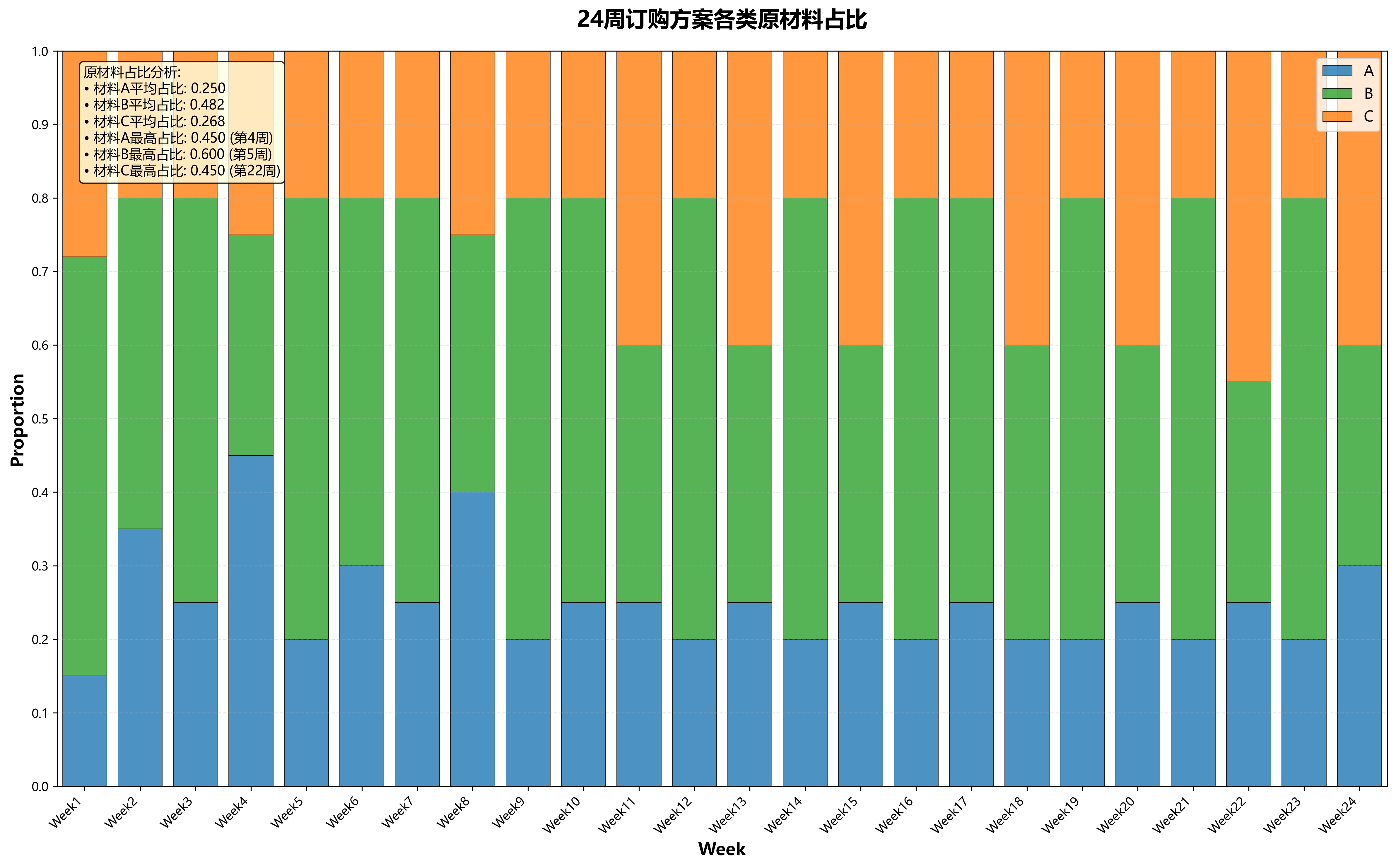


------std::lock_guard)


:Model抽象层 - “驯服”天下AI的“紧箍咒”)


:polygonOffsetFactor工作原理大揭秘)


